Contents
Scroll to:
https://doi.org/10.17073/0368-0797-2026-1-84-90
Scroll to:
Mathematical model of the shrinkage process in a continuously cast slab during its cooling and solidification is proposed. The model is based on solution of the equation of non-stationary thermal conductivity and provisions of the theory of a quasi-equilibrium two-phase zone. Unlike previously proposed models of the slab cooling and solidification process, the proposed one takes into account the dependence of thermal properties of the steel on temperature, as well as such features as chemical composition of the cast steel, geometric shape of the slab cross-section and the process parameters of casting rate and intensity of slab cooling in the secondary cooling zone. The model implements the solution of the heat conductivity equation using the finite difference method, approximation of partial derivatives is performed according to an explicit scheme. During modeling, the temperature field is calculated in the computational domain, which is a quarter of the slab cross-section. In this case, the boundary conditions in the mold and cooling sections of the secondary cooling zone of continuous casting machine are taken into account. The model also implements calculation of the total shrinkage in the slab from the moment of crystallization and also can be used to calculate the shrinkage cavity depth formed in the slab after casting. The model adequacy is confirmed by verification performed by comparing the modeling data with experimental data on the shrinkage cavity depth. Dependence of the modeling accuracy on the number of computational grid nodes is also revealed. The presented model allows calculating the shrinkage cavity depth and developing recommendations for adjusting the mold taper and the parameters of continuous casting machine roller guide depending on the amount of metal shrinkage during cooling and solidification of continuously cast slabs.
Chuev A.A., Lukin S.V. Modeling of shrinkage processes in slabs during steel casting in continuous casting machines. Izvestiya. Ferrous Metallurgy. 2026;69(1):84-90. https://doi.org/10.17073/0368-0797-2026-1-84-90
Introduction
One of the most important technological processes in modern metallurgy is continuous casting. During the cooling and solidification of a slab in a continuous casting machine (CCM), metal shrinkage occurs, resulting in the formation of a shrinkage cavity in the upper part of the final slab. Of particular interest is the development of a method for calculating the shrinkage of a continuously cast slab in the mold and the secondary cooling zone (SCZ) of a CCM, as well as determining the slab dimensions with shrinkage taken into account. A number of mathematical models describing the processes of slab cooling and metal shrinkage have been developed. Research on this topic began in the 1970s. For example, study [1] was devoted to calculating shrinkage during solidification of a billet with a circular cross-section. Subsequently, the developed models became more sophisticated, incorporating hydrodynamic phenomena in the liquid phase [2], more detailed descriptions of slab bulging [3], phase transformations during casting [4], thermomechanical phenomena [5], heat transfer in the secondary cooling zone [6], and other factors.
The development of a predictive shrinkage model would make it possible to account for the influence of shrinkage on technological parameters such as mold taper and the roller gap in the SCZ. In study [7], an attempt was made to predict the “ideal” mold taper using a two-dimensional mathematical model. Attempts were also made to develop a model that takes into account the carbon content in steel [8].
In Russian research, particular attention has been given to the works of Dyudkin D.A. [9] and Samoylovich Yu.A. and Kabakov Z.K. [10; 11], who developed a universal model describing the cooling and solidification of a continuously cast slab. This model subsequently formed the basis for numerous further developments, including models of slab surface layer formation [12], continuous slab deformation [13], and the secondary cooling zone (SCZ) system of the CCM [14; 15], among others.
Most proposed models assume that the thermal properties of the metal are independent of temperature. In many cases, these properties are taken as constant for both the solid and liquid phases. When reliable temperature-dependent data are unavailable, the properties are typically estimated by linear interpolation. Moreover, the calculated shrinkage parameters strongly depend on the selected numerical method: study [16] shows that results obtained using different models for identical input data may differ by more than a factor of two
Thus, the existing models of shrinkage processes are not universal and remain imperfect, since they do not account for all features of slab solidification and cooling in a CCM. Therefore, there is a need to develop a more comprehensive mathematical model of shrinkage processes in continuously cast slabs.
Fundamental theoretical provisions
The mathematical model of cooling and solidification of a continuously cast slab is based on the solution of the transient heat conduction equation:
| \[\begin{array}{c}{c_{{\rm{eff}}}}\rho \left( {\frac{{\partial T}}{{\partial t}} + v\frac{{\partial T}}{{\partial z}}} \right) = \frac{\partial }{{\partial x}}\left( {\lambda \frac{{\partial T}}{{\partial x}}} \right) + \frac{\partial }{{\partial z}}\left( {\lambda \frac{{\partial T}}{{\partial z}}} \right) + \Theta (x,y,t),\\0 \le t \le {t_{\rm{c}}},{\rm{ }}0 \le x \le B,{\rm{ }}0 \le z \le h,\end{array}\] | (1) |
where ceff is the effective heat capacity of steel; ρ is the steel density; λ is the thermal conductivity of the melt; B is half of the slab thickness, m; h is the slab height, m; v is the slab withdrawal rate along the vertical axis, m/min; Θ is the heat source of superheated metal in the region influenced by the casting jet.
| \[{c_{{\rm{eff}}}} = \left\{ \begin{array}{l}{c_{\rm{m}}},{\rm{ }}T < {T_{\rm{s}}},{\rm{ }}T > {T_{\rm{l}}};\\{c_{\rm{m}}} - L\frac{{d\psi }}{{dT}},{\rm{ }}{T_{\rm{s}}} \le T \le {T_{\rm{l}}},\end{array} \right.\] | (2) |
where cm is the molecular heat capacity of the alloy; Тs and Тl are the solidus and liquidus temperatures, respectively; L is the latent heat of solidification of the metal in the solid–liquid (two-phase) zone; \(\frac{{d\psi }}{{dT}}\) is the rate of phase transformation during equilibrium solidification of the binary alloy.
Since metal solidification depends on the percentage carbon content, establishing the temperature dependence ceff (T) requires consideration of the Fe–C phase diagram, particularly its high-temperature part (Fig. 1).
Fig. 1. High-temperature part of Fe – C diagram |
The diagram shown in Fig. 1 identifies three steel groups: I – [% С] ≤ 0.1; II – 0.1 < [% С] ≤ 0.16; III – 0.16 < [% C] ≤ 0.5. For each group, the temperature dependence ceff (T) was determined, where:
| \[{c_I}(T) = {c_M} - \left\{ \begin{array}{l}0,{\rm{ }}T < {T_{NJ}};{\rm{ }}{T_{NH}} \le T < {T_{AH}};{\rm{ }}T \ge {T_{AB}},\\{L_{{\rm{l}} - \delta }}\frac{{d{\psi _\delta }}}{{dT}},{\rm{ }}{T_{AH}} \le T < {T_{AB}};\\{L_{\delta - \gamma }}\frac{{d{\psi _\gamma }}}{{dT}},{\rm{ }}{T_{NJ}} \le T < {T_{NH}},\end{array} \right.\] | (3) |
where Ll – δ is the latent heat of the liquid → δ-ferrite transformation; Lδ – γ is the latent heat of the δ-ferrite → austenite transformation; ψδ is the volume fraction of δ-ferrite in the elementary volume of the “liquid + δ-ferrite” mixture; ψγ is the volume fraction of austenite in the “δ-ferrite + austenite” mixture; \(\frac{{d{\psi _\delta }}}{{dT}}\) and \(\frac{{d{\psi _\gamma }}}{{dT}}\) are the rates of formation of δ-ferrite and austenite, respectively.
| \[\begin{array}{c}{c_{II}}(T) = {c_M} + \delta (T - {T_J}){Q_1} - \\ - \left\{ \begin{array}{l}0,{\rm{ }}T < {T_{NJ}};{\rm{ }}T \ge {T_{AB}},\\{L_{{\rm{l}} - \delta }}\frac{{d{\psi _\delta }}}{{dT}},{\rm{ }}{T_J} \le T < {T_{AB}};\\{L_{{\rm{l}} - \gamma }}\frac{{d{\psi _\gamma }}}{{dT}},{\rm{ }}{T_{NJ}} \le T < {T_J},\end{array} \right.\end{array}\] | (4) |
where δ(T) – is the Dirac delta function, which was approximated by the expression \(\delta (x) \approx \frac{1}{{a\sqrt \pi }}{e^{ - {{\left( {\frac{x}{a}} \right)}^2}}};\)
| \[\begin{array}{c}{c_{III}}(T) = {c_M} + \delta (T - {T_J}){Q_2} - \\ - \left\{ \begin{array}{l}0,{\rm{ }}T < {T_{JE}};{\rm{ }}T \ge {T_{AB}},\\{L_{{\rm{l}} - \delta }}\frac{{d{\psi _\delta }}}{{dT}},{\rm{ }}{T_J} \le T < {T_{AB}};\\{L_{{\rm{l}} - \gamma }}\frac{{d{\psi _\gamma }}}{{dT}},{\rm{ }}{T_{JE}} \le T < {T_J}.\end{array} \right.\end{array}\] | (5) |
Similarly, the temperature dependences of the effective thermal conductivity λeff (T) and the density ρ(T) were determined.
The calculation of the linear shrinkage coefficient αl (T) was carried out based on the obtained values of the thermal parameters. Since the temperature dependence of the specific volume V(T) in the Fe–C system is strongly influenced by the carbon concentration, it can be concluded that a similar dependence also applies to linear shrinkage. In the proposed model, the coefficient αl (T) is calculated using the expression for volumetric shrinkage given in [17]:
| \[{\alpha _V}(T) = \frac{{dV(T)}}{{dT}}\frac{1}{{V(T)}},\] | (6) |
where V(T) is the temperature-dependent specific volume of the alloy; \(\frac{{dV(T)}}{{dT}}\) is the temperature derivative of the specific volume.
The calculated values of the volumetric shrinkage coefficient αV (T) are subsequently used to determine the shrinkage cavity depth [18].
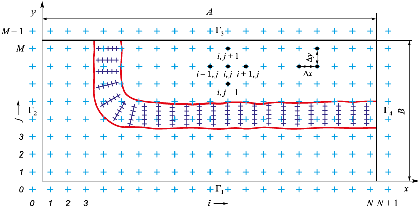
To solve equation (1), the finite difference method (FDM) was applied using an explicit scheme for approximating the partial derivatives, with the introduction of fictitious nodes that allow more accurate approximation of boundary derivatives with respect to x and y. The computational domain represents one quarter of the slab cross-section (Fig. 2). The number of nodes in the region 0 ≤ x ≤ A is taken as N, and in the region 0 ≤ x ≤ B as M.
Fig. 2. Scheme of discretization of the computational domain. |
At the initial time, the temperature is assumed to be uniform and equal to the liquidus temperature:
| T(0, x, y) = Tl = const. | (7) |
The boundary conditions on boundaries Г3 and Г4 are:
| \(\lambda \frac{{\partial T}}{{\partial w}} = 0,\) where w = x, y. | (8) |
The boundary conditions for the cooling zones along boundary Γ1 are defined as follows:
– in the mold:
| q = αm (Ts – Tw ), | (9) |
where αm is the heat transfer coefficient in the mold; \(q = - \lambda \frac{{\partial T}}{{\partial w}},\) where w = x, y is the heat flux from one face of the slab;
– in the i-th SCZ section:
| \(\lambda \frac{{\partial T}}{{\partial w}}\) = αi (Ts – Tam ), where w = x, y; | (10) |
– air cooling:
| \[\begin{array}{c}\lambda \frac{{\partial T}}{{\partial w}} = {\alpha _{\rm{l}}}\left( {{T_{{\rm{s}}}} - {T_{{\rm{am}}}}} \right),\\{\alpha _{\rm{l}}} = {\sigma _{\rm{l}}}\left( {T_{{\rm{s}}}^2 + T_{{\rm{am}}}^2} \right)\left( {{T_{{\rm{s}}}} + {T_{{\rm{am}}}}} \right) + {\alpha _{\rm{c}}},\end{array}\] | (11) |
where αl is the heat transfer coefficient in the i-th SCZ section; Тs is the slab surface temperature; Тw is the temperature of the cooling water in the mold; Тm is the temperature of the working (copper) wall of the mold; Тam is the ambient temperature; σl is the radiation coefficient; αl is the effective heat transfer coefficient during air cooling; αc is the convective heat transfer coefficient Boundary conditions on Г2 are specified in a similar manner.
The procedure for calculating linear shrinkage is as follows. The calculation is performed for one quarter of the slab cross-section, and the solidus isotherm is taken as the boundary of complete solidification. In [19], an expression was obtained for the relative strain rate of the solid shell:
| \[\eta = \frac{1}{\xi }\int\limits_0^\xi {{\alpha _l}(T)\dot Tdx} ,\] | (12) |
where ξ is the thickness of the solid shell; αl (Т) is the linear shrinkage coefficient of steel; \(\dot T\) is the temperature change rate at point x at time t.
After integrating this expression over the width of the face, the strain rate expressions for the wide face (ηwf ) and narrow face (ηnf ) of the slab are obtained. The total deformation of the faces from the onset of solidification is then determined:
| \[{\eta _{{\Sigma _{{\rm{wf}}}}}} = \int\limits_0^t {\frac{1}{{{\xi _{{\rm{wf}}}}}}\int\limits_0^{A(t)} {\int\limits_0^{{\xi _{{\rm{wf}}}}} {{\alpha _l}(T)\dot Tdydxdt} } } ;\] | (13) |
| \[{\eta _{{\Sigma _{{\rm{nf}}}}}} = \int\limits_0^t {\frac{1}{{{\xi _{{\rm{nf}}}}}}\int\limits_0^{B(t)} {\int\limits_0^{{\xi _{{\rm{nf}}}}} {{\alpha _l}(T)\dot Tdxdydt} } } ,\] | (14) |
where ξшг and ξуг are the thicknesses of the solidified layer at the wide and narrow faces, respectively, mm; αl (T) is the linear shrinkage coefficient, °C–1; \(\dot T\) is the rate of temperature decrease/increase at point x at time t, °C/s.
Then, the slab thickness and width during solidification are determined as follows
| \[x_A^{n + 1} = 2A\left( {1 - \eta _{{\Sigma _{{\rm{wf}}}}}^{n + 1}} \right);\] | (15) |
| \[x_B^{n + 1} = 2B\left( {1 - \eta _{{\Sigma _{{\rm{nf}}}}}^{n + 1}} \right).\] | (16) |
Verification
The model was implemented as a computer program. The following input data were used in the simulations: slab thickness B = 0.2 m, slab height h = 6.5 m, initial temperature T0 = 1520 °С, ambient temperature Тam = 30 °С, liquidus temperature Тl = 1500 °С, solidus temperature Тs = 1450 °С, number of nodes across the thickness M = 20, number of nodes across the height N = 2500, casting rate v = 0.4 m/min, and cross-section 200×1200 mm. The mold length, SCZ section lengths, and the heat transfer coefficients for the individual sections are given in Table 1.
Table 1. Size of crystallizer and sections of secondary cooling zone
| ||||||||||||||||||||||||||||||||||||||||||
Verification was performed by comparing the calculated shrinkage cavity depth with the experimental data reported in [20]. According to [20], the mean cavity depth for a sample of 26 slabs is 0.353 m. In turn, the shrinkage cavity depth obtained in the simulation was 0.35 m (Fig. 3).
Fig. 3. Calculated shrinkage cavity profile |
During verification, the dependence of the relative modeling error on the number of grid nodes along the height N and thickness M was also identified (see Tables 2 and 3).
Table 2. Dependence of shrinkage cavity depth on the number of nodes by height
Table 3. Dependence of shrinkage cavity depth on the number of nodes by thickness
|
Tables 2 and 3 show that modeling accuracy increases with increasing numbers of nodes along the height and thickness, reaching an acceptable level of <5 % at N = 2500 and M = 20.
Conclusions
A mathematical model of the shrinkage process in a continuously cast slab has been developed. Its distinctive feature is the incorporation of temperature-dependent thermal properties of the metal and technological casting parameters.
Model verification confirmed the agreement between the simulation results, theoretical calculations, and experimental data.
The modeling accuracy increases with increasing numbers of computational grid nodes along the height N and thickness M, with M having a stronger effect on the modeling accuracy.
The proposed model can be used to improve continuous casting technology.
1. Bauman H.G., Schafer G. Beitrag zur Berechnung der Kontraktion von Stahl Während seiner Erstarrung. Archiv für das Eisenhüttenwesen. 1970;41(12):1111–1115. (In Germ.).
2. Telejko T., Malinowsky Z., Rywotycki M. Analysis of heat transfer and fluid flow in continuous steel casting. Archives of Metallurgy and Materials. 2009;54(3):837–844.
3. Wu D., Li J., Qin Q., Ma T. Research on creep material models and bulging of cast slab. In: 2010 Int. Conf. on Mechanic Automation and Control Engineering, Wuhan, China; 2010:5536–5539. https://doi.org/10.1109/MACE.2010.5535615
4. Chimani C.M., Resch H., Mörwald K., Kolednik O. Precipitation and phase transformation modelling to predict surface cracks and slab quality. Ironmaking & Steelmaking. 2005;32(1):75–79. https://doi.org/10.1179/174328105X15814
5. Zappulla M.L.S., Thomas B.G., Hibbeler L.C. Effect of grade on thermal-mechanical behavior of steel during initial solidification. Metallurgical and Materials Transactions A. 2017;48(8):1–17. https://doi.org/10.1007/s11661-017-4112-z
6. Assuncao C., Tavares R., Oliveira G. Improvement in secondary cooling of continuous casting of round billets through analysis of heat flux distribution. Ironmaking & Steelmaking. 2015;42(1):1–8. https://doi.org/10.1179/1743281214Y.0000000190
7. Li C., Thomas B.G., Storkman W.R., Moitra A. Ideal mold taper prediction using CON2D. In: Proceedings of the 9th Int. Iron and Steel Congress, Nagoya, Japan, Iron & Steel Inst. Japan, Tokyo.1999;3:348–355.
8. Zhu L.-G., Kumar R.V. Shrinkage of carbon steel by thermal contraction and phase transformation during solidification. Ironmaking & Steelmaking. 2007;34(1):71–75. https://doi.org/10.1179/174328106X118143
9. Dyudkin D.A., Krupman L.I., Maksimenko D.M. Shrinkage Cavities in Steel Ingots and Billets. Moscow: Metallurgiya; 1983:137. (In Russ.).
10. Samoilovich Yu.A., Kabakov Z.K. Taking into account the effect of stress relaxation when determining thermal stresses in a casting. In: Combustion, Heat Transfer and Heating of Metal: Proceedings. Moscow: Metallurgiya; 1973;(24): 100–113. (In Russ.).
11. Samoilovich Yu.A., Kabakov Z.K., Goryainov V.A., Perminov V.P., Podorvanov A.G., Sakhnov B.I. Application of mathematical models to study the processes of solidification and cooling of continuous steel ingots of rectangular cross-section. In: Nepreryvnaya Razlivka Stali. Moscow: Metallurgiya; 1974;(2):44–49. (In Russ.).
12. Khasin G.A. On mathematical modeling of formation of ingot surface layers. Izvestiya. Ferrous Metallurgy. 1987;30(8):133–135. (In Russ.).
13. Danilov V.L., Korablin A.I. Mathematical model of deformation of continuously cast steel slabs. BMSTU Journal of Mechanical Engineering. 1989;(12):142–145. (In Russ.).
14. Yaukhola M., Kivelya E., Konttinen Yu., Laitinen E. Dynamic model of the secondary cooling zone cooling system for continuous casting machines. Stal’. 1995;(2):25–29. (In Russ.).
15. Devyatov D.Kh., Panteleev I.I. Determination of heat transfer coefficients in CCM secondary cooling zone using identifiable mathematical model. Izvestiya. Ferrous Metallurgy. 1999;42(8):62–65. (In Russ.).
16. Meng Y., Li C., Parkman J., Thomas B.G. Simulation of shrinkage and stress in solidifying steel shells of different grade. In: Solidification Processes and Microstructures: A Symposium in Honor of Wilfried Kurz edited by M. Rappaz TMS (The Minerals, Metals & Materials Society), Charlotte, NC. 2004:33–39.
17. Thomas B.G., Ojeda C. Ideal taper prediction for slab casting. In: 2003 ISSTech Steelmaking Conf., Indianapolis, IN, USA, April 27-30, 2003, ISS-AIME, Warrendale, PA. 2003:295–308.
18. Kabakov Z.K., Gabelaya D.I., Chuev A.A. Mathematical model of formation of shrinkage cavity of continuously cast billet on continuous casting machine. In: 13th Int. Sci. and Tech. Conf. “INFOS-2022”: Proceedings. Vologda: VSU; 2022:14–18. (In Russ.).
19. Samoilovich Yu.A., Goryainov V.A., Krulevetskii S.A., Kabakov Z.K. Thermal Processes in Continuous Steel Casting. Moscow: Metallurgiya; 1982:152. (In Russ.).
20. Dyudkin D.A. Conditions for forming the end portion of a continuous ingot. In: Proceedings of the III Conf. on the Ingot “Problems of the Steel Ingot”. Moscow: Metallurgiya; 1969:375–381. (In Russ.).
Anton A. Chuev, Senior Lecturer of the Chair of Mathematics and Informatics
5 Lunacharskogo Ave., Cherepovets, Vologda Region 162600, Russian Federation
Sergei V. Lukin, Dr. Sci. (Eng.), Prof. of the Chair Thermal Power and Heat Engineering
5 Lunacharskogo Ave., Cherepovets, Vologda Region 162600, Russian Federation
Chuev A.A., Lukin S.V. Modeling of shrinkage processes in slabs during steel casting in continuous casting machines. Izvestiya. Ferrous Metallurgy. 2026;69(1):84-90. https://doi.org/10.17073/0368-0797-2026-1-84-90
 Email this article (Login required)
Email the author (Login required)
Email this article (Login required)
Email the author (Login required) Publishing House of National University of Science and Technology "MISIS"
4, Leninskii prospekt, Moscow, 119991, Russia
Phone: +7 (495) 638-44-11, +7 (495) 784-58-66
E-mail: fermet.misis@mail.ru