Shewhart control charts – A simple but not easy tool for data analysis

All models are wrong,
but some are useful.
George Box

Introduction

Shewhart Control Charts (ShCCs) are widely recognized as a principal tool evaluating process stability at almost all fields of human activity. These charts were developed nearly a century ago by Walter Shewhart, who is acclaimed for his significant contributions to the field of quality management. His famous works, published in 1931 and 1939, have been reissued in facsimile editions by the American Society for Quality in 1980 and 1986, respectively [1; 2]. W. Edwards Deming, a close collaborator and friend of Shewhart, wrote a brief foreword to the 1939 publication, concluding with the following words: “Another half-century may pass before the full spectrum of Dr. Shewhart’s contributions has been revealed in liberal education, science, and industry” [2]. This paper aims to address some of the obstacles encountered in achieving the vision articulated by Deming. Firstly, we will examine the extent to which ShCCs have been adopted globally. Then, we will explain why, despite its apparent simplicity, the ShCCs remain a challenging tool to apply effectively. This analysis will draw upon both historical studies and recent research findings.

Current status of ShCCs use

Upon first review, the use of ShCCs seems to be quite straightforward, finding application across diverse sectors such as metallurgy, automotive, semiconductor manufacturing, aviation, agriculture, government, healthcare, and education.

ShCCs, as part of statistical process control (SPC), are widely cited in scholarly works [3 – 6], ranging from foundational texts that are considered classics to contemporary studies [7 – 10]. They are also supported by international standards like those mentioned in [11] and various online resources that provide instructions for their use.

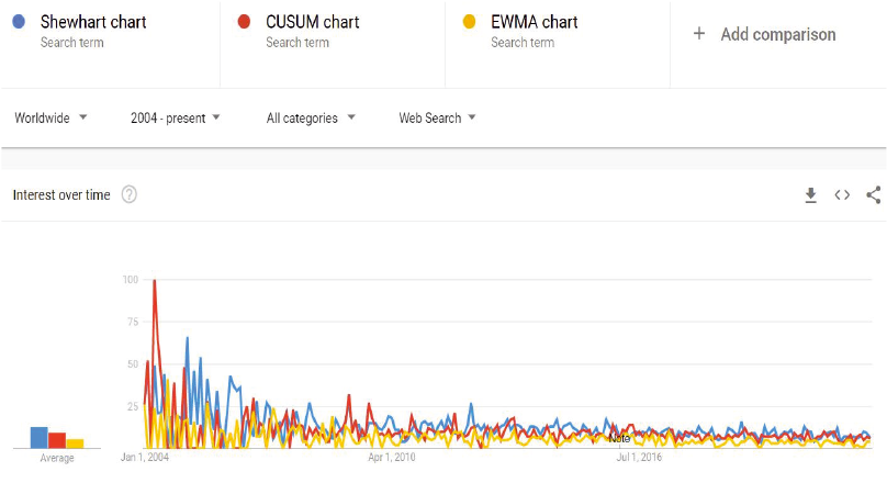
However, there are at least two problems that cannot let us say “Everything is OK!” in the area of ShCCs. One notable issue is the declining interest in ShCCs among statisticians and industry professionals, as evidenced by the information depicted in Fig. 1 and a decrease in the volume of related scholarly publications in esteemed journals. The paper [12] recently addressed this topic. Part of this issue can be attributed to the formal and bureaucratic procedures for implementing ShCCs mandated by some international standards. Another concern is the noticeable scarcity of new research on ShCCs that goes beyond the conventional models of basic control charts. Our critique does not concern the creation of new types of charts – there is plenty of innovation in that area. Instead, we highlight the need for expanding the applications of charts beyond the traditional assumptions of ShCCs theory. Here are a few uncommon examples of such research. In 2011, the study “Assignable causes of variation and statistical models: another approach to an old topic” was published [13]. The authors, one of whom is a co-author of this article, suggested dividing the assignable causes of variation into two categories: those caused by an intervention with the same distribution function (DF) as the original process and those with a different DF. While the former approach has been used in all prior studies, the latter presents an operating characteristic (the probability of a point exceeding the chart limits) that significantly deviates from what is described in textbooks. The 2017 publication [14] brought up the significant issue regarding the sequence of points, highlighting that processes with random data are nearly non-existent. However, current ShCCs theory assumes that process data are completely random. In 2021, a paper was released detailing the effects of a transient shift in the process mean on ShCCs behavior [15]. The findings demonstrated that in cases of a transient shift, the chart for the mean might become less effective compared to the chart for individual values. This contradicts all standard SPC guidelines. These examples represent just a small fraction of the potential for broadening the scope of traditional ShCCs applications by challenging the assumptions that have underpinned standard models for decades.

This work further extends the exploration of traditionally overlooked conditions. This time, we will move beyond the common assumption that process parameters are normally distributed and will discuss several implications of this departure. Additionally, we will examine various types of assignable causes of variation and their effects on the utilization of ShCCs.

Effects of non-normal distribution on ShCCs performance

This section is divided into two parts. Firstly, we will examine whether measurement results are always normally distributed. Secondly, we will show how the limits of ShCCs change when the DF is non-normal and will describe the most user-friendly method to address this issue.

Are the measurement results always normally distributed? This assumption is widely accepted by numerous authors, texts, and even standards. For example, the standard [11] articulates: “According to this standard, the application of control charts for quantitative data presumes that the characteristic under surveillance adheres to a normal (Gaussian) distribution, and deviations from this norm can influence the effectiveness of the charts. The coefficients for calculating control limits are predicated on a normal distribution of characteristics. Given that control limits frequently serve as empirical benchmarks in decision-making, reasonably small deviations from normality are conceivable. The central limit theorem posits that sample mean values tend toward a normal distribution, even if individual observations deviate from this norm. This supports the premise of normality for X-charts, even with sample sizes as small as 4 or 5 units. However, for assessments of process capabilities using individual observations, the actual distribution is crucial. Although the distributions of ranges and standard deviations deviate from normality, the calculation of control limits for range and standard deviation charts initially assumed normality. Nevertheless, minor deviations from a normal distribution in process characteristics should not prevent the employment of such charts for empirical decision-making” (emphasis ours).

But what exactly constitutes “reasonably small deviations from normality” or “minor deviations”? These terms do not provide a clear definition of what extent of change in the distribution law is deemed significant [16] Recent findings [17] offer an operational definition for these terms and an algorithm for constructing ShCCs under the clear presence of non-normal DF.

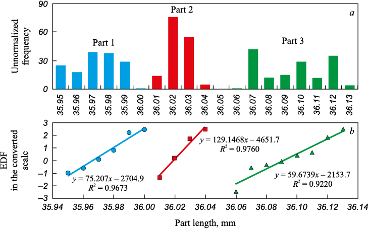
A common misconception about the universal applicability of the normal law is the belief that measurement results always follow a Gaussian curve. To empirically test this assumption, three parts from the same process but from different points within the tolerance range were each measured 150 times using the same instrument. The outcomes are depicted in Fig. 2. ShCCs for the parts indicated that the processes for the first and second parts were stable, whereas for the third part, just three distinct categories were identified. All histograms were noticeably non-normal, and the hypothesis of normality was conclusively disproven through the testing procedure outlined in [18]. Therefore, it is reasonable to argue that the results of repeated measurements might not adhere to the normal distribution, akin to the measurement outcomes of various objects.

How does non-normality of DFs affect ShCCs coefficients? Numerous DF processes markedly deviate from the Gaussian law. The question arises: how can the stability of such processes be assessed when a control chart is the sole instrument for ascertaining process stability? The study [17] offers an exhaustive literature review alongside the outcomes of simulating asymmetric data. It contrasts the results of analyzing non-normal data through both the conventional method and the algorithm introduced in [17]. The conventional method adheres to the declaration cited from the standard [11]. Yet, what will empirical evidence disclose?

Initially, 400 samples of random numbers following an exponential distribution with the parameter λ = 0.01 were generated, with each sample comprising 400 points. This was achieved by generating random numbers from a uniform distribution function using Excel, and then transforming these numbers by taking their logarithms and multiplying by (–100) to produce a set of exponentially distributed data samples.

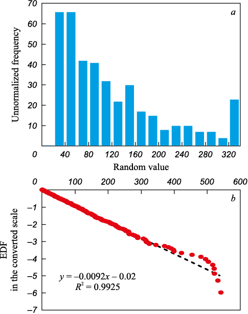
The histogram for one of the generated samples is displayed in Fig. 3, a. Fig. 3, b illustrates the empirical DF on a probability plot for the exponential distribution. Both sections of Fig. 3 affirm that the sample’s point distribution closely aligns with an exponential distribution¹. The descriptive statistics parameters are as follows: the mean is 105.5; the standard deviation is 105.0; skewness is 1.82; kurtosis is 3.78 (Note: Excel 2013 calculates excess kurtosis); the minimum value is 0.51; the maximum value is 541.4; the median is 73.9; the first quartile is 31.1; the third quartile is 142.8; and the upper boundary for extreme outliers is determined to be 477.87, which allowed for the identification of eight extreme outlier (EO)² points (these are clearly visible in Fig. 3, b).

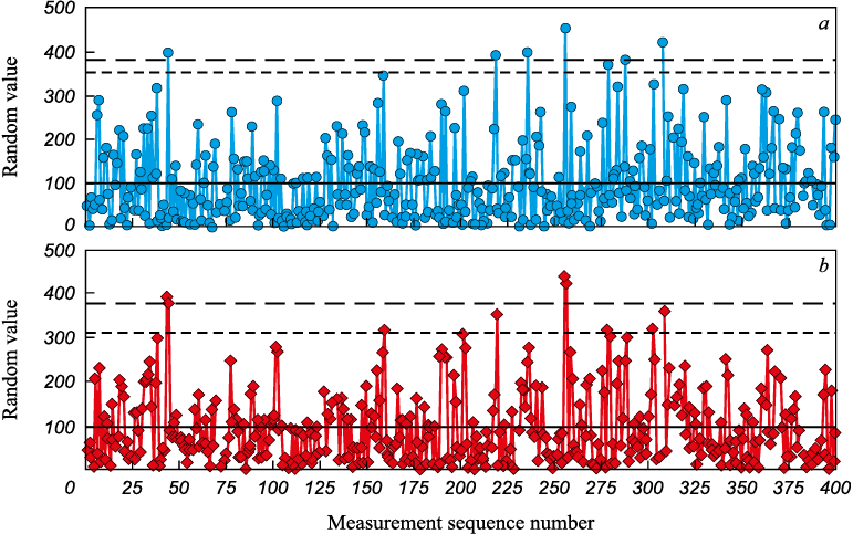
After removing EOs, the control chart for individual values and moving range (x-mR) was created using standardized values of ShCCs coefficients [19]: E₂ = 2.66; D₄ = 3.27. The resulting x-mR chart is depicted in Fig. 4, with the control limits illustrated by dashed lines. The process is identified as unstable, as seven points (representing 1.8 % of the total) in the chart for individual values (x) and nine points (accounting for 2.2 %) in the chart for moving range (mR) exceed the upper control limit (UCL). However, based on the findings in [17], the coefficient d₂ for an exponential DF should be 2.99, not 2.66. The limit, recalculated using the revised coefficients, is also displayed in Fig. 4, marked by long dashes. It is observed that with this adjustment, only six points in the x-chart exceed the UCL. Similarly, on the mR chart, the count of points exceeding the upper control limit dropped to four from nine, nearly halving the number of signals. Therefore, in this scenario, the incidence of false alarms was reduced by 14 % on the chart for individual values and by 44 % on the moving range chart. Using a chart for medians, instead of means, would have produced identical outcomes.

In a second example, monthly data on the number of technological violations at a large mining and processing plant are presented in a Table.

The question arises: Should the increased value in September be considered an assignable cause of variation, or in other words, is the process stable?

To address this, an x-mR chart needs to be constructed. Using the traditional methodology for creating ShCCs, we obtain the following parameters for the chart: the center line (CL) is 20.7; the mean moving range (MMR) is 13.2; the UCL is 55.7. With the September value exceeding the UCL, it suggests that the process is unstable, and an interference cause should be identified. However, this conclusion comes from the traditional approach. The critical inquiry then is whether employing the traditional method was appropriate for this analysis.

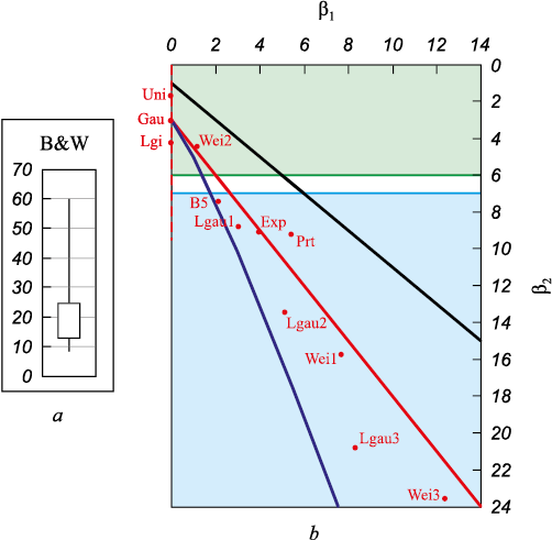
Given the small sample size, a box-and-whisker plot was chosen over a histogram (Fig. 5). This plot clearly indicates that the data are asymmetric. The question then arises: Is this level of deviation from normality significant? One method to address this question involves calculating the skewness and kurtosis values. Excel reports skewness as 2.0 and kurtosis as 4.7. However, Excel calculates excess kurtosis, meaning the actual kurtosis value is 7.7. According to [17], for kurtosis values exceeding 7.0 – when the specific DF matching our data is unknown – it is recommended to use the coefficient value for the closest point on the plane of Pearson curves (Fig. 5, b). For the data in question, the nearest point is B5, corresponding to the Barr DF. The E₂ value for this DF = 2.81 and adjusted UCL = 57.7 [17]. Therefore, the value for September still exceeds the UCL, leaving the assessment of process stability unchanged. However, if the data had been closer to an exponential distribution (for example, if the kurtosis were about 9), then the adjusted coefficient would be 2.99, the adjusted UCL would become 60.1, and the process would be considered stable, indicating no assignable causes of variation on the chart.

These examples demonstrate an important aspect of the ShCCs that is often overlooked by many scholars and not fully grasped by practitioners: ShCCs are the tool that necessitates direct interaction with the process. The construction of the ShCCs cannot be entirely reduced to an algorithm [20]. To use ShCCs effectively, one must possess a deep understanding of the process’s nuances as well as a solid grasp of control chart theory. The authors claim that the absence of such a synergistic approach is likely the main reason why this potent tool frequently fails to give a practitioner a helping hand.

Reflections on process stability and analysis techniques

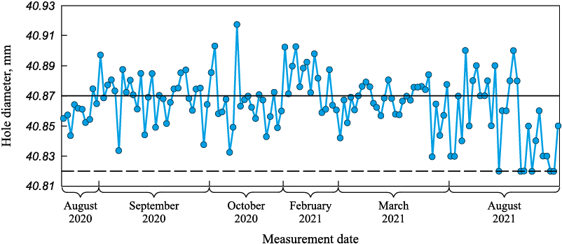
As mentioned earlier, the Shewhart control chart is the only tool for determining process stability. However, different types of instability necessitate varied responses. Let us examine the process shown in Fig. 6, which comes from a real case with data collected from a machine-building plant in Russia. The manufacturing technology for the part being monitored did not change at all during the period of observation, and the production system remained the same. Fig. 6 illustrates that all manufactured parts met tolerance requirements (there were no rejections), which means the customer’s standards were met. From the perspective of process stability, let us examine the subject first through the eyes of an engineer unfamiliar with SPC procedures, whom we will refer to as a novice, and then from the standpoint of a user well-versed in SPC methods, referred to as an expert.

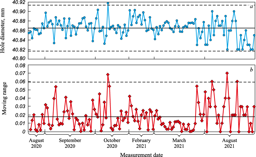
A novice, without hesitation, will analyze all available data and derive the x-mR chart as illustrated in Fig. 7. The CL will be calculated at 40.865, the UCL at 40.913, and the lower control limit (LCL) at 40.817. This chart suggests that the process exhibits instability (with one point exceeding the UCL and four points surpassing the UCLmR on the mR chart). Alternatively, it could be interpreted that the process was stable during August and September 2021 and in March 2022 but entered a phase of instability in October 2021 and again in March 2022. For the novice, computing the Process Capability Index (PCI) also presents no challenge: C_p will be equal to 1.04 (0.1 divided by 6 sigma, with sigma being the mean moving range divided by d₂). A C_p value of 1.04 equates to a potential non-conformity level (NL) of 0.18 % or a process yield (PY) of 99.82 %.

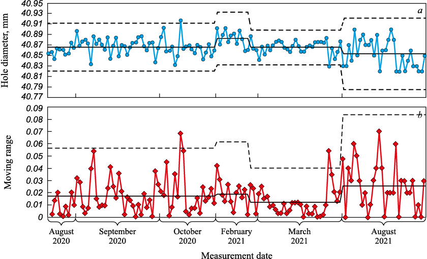
An expert would observe that the process is distinctly heterogeneous and recommend its division into homogeneous segments for more accurate analysis. This approach of stratification is depicted in Fig. 8, where four segments are identified, each with distinct CL values and control limits:

Section 1: August – October 2020.

CL = 40.8665; CLmR = 0.0173; UCL = 40.9124; LCL = 40.8206; UCLmR = 0.0564.

Section 2: February 2021.

CL = 40.8830; CLmR = 0.0189; UCL = 40.9331; LCL = 40.8329; UCLmR = 0.0616.

Section 3: March 2021.

CL = 40.8662; CLmR = 0.0123; UCL = 40.8990; LCL = 40.8334; UCLmR = 0.0403.

Section 4: end of March and August 2021.

CL = 40.8537; CLmR = 0.0256; UCL = 40.9218; LCL = 40.7856; UCLmR = 0.0837.

The PCI values for each section are as follows: section 1: C_p = 1.09; section 2: C_p = 1.00; section 3: C_p = 1.53; section 4: C_p = 0.73. Calculating NL for each section yields values ranging from 4.7 to 27,525 ppm. Given such a jaw-dropping difference, two pressing questions arise:

– Which analytical method is most appropriate for process improvement?

– How should the stability of such a process be interpreted?

Let us address the latter question first.

Various forms of process instability

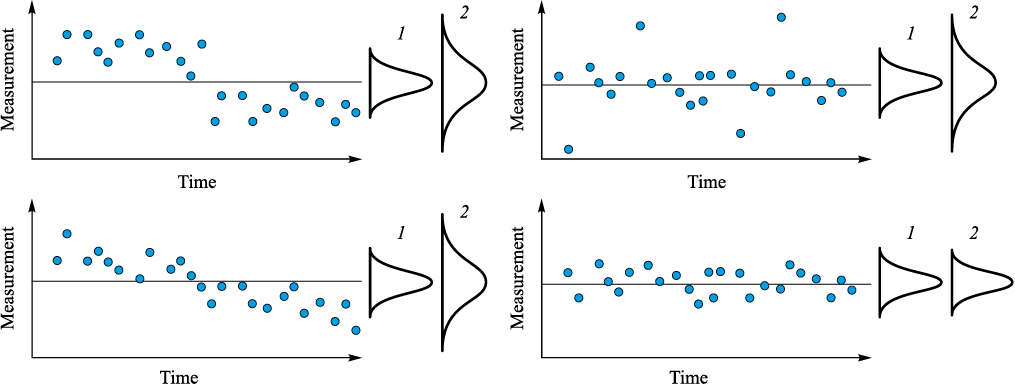
It’s clear that instability can manifest itself in various forms. Dr. Deming highlighted this distinction in his introduction to Shewhart’s 1939 book [2]: “A significant contribution of the control chart lies in its ability to methodically differentiate variation sources into two categories: (1) systemic causes (“change causes”, as Dr. Shewhart termed them), which fall under management’s purview; and (2) assignable causes, referred to by Deming as “special causes”, which are tied to transient events and can typically be identified and eliminated by the process expert. A process is deemed to be in statistical control when it is free from the impact of special causes. Such a process, once in statistical control, exhibits predictable performance”. Fig. 9, drawn from [21], explores various special causes of variation identified in different processes. In three of the four illustrations, a step change in the mean, outliers, and a drift in the mean are evident. However, only the illustration depicting outliers aligns with the “ephemeral event”. Deming mentioned in the previously quoted text. Deming wasn’t alone in this viewpoint. W. Woodall in the paper [22] provides this definition: “Common cause variation is attributed to the intrinsic characteristics of the process and cannot be modified without altering the process itself. “Assignable (or special) causes” of variation are unusual shocks or other disruptions to the process, the causes of which can and should be removed”.

The two left images in Fig. 9 indicate that the process underwent a change due to some cause. The question arises: Is this cause common or assignable? Given that common causes are regarded as “constant” (a term used by Shewhart in his works [1; 2]) and inherent to the process itself, the causes for the variation seen in the left part of Fig. 9 should be classified as assignable. However, these causes differ from outliers and other transient events. Thus, it appears suitable to acknowledge different types of assignable (special) causes. In reference [13], the authors suggest introducing two types of assignable causes of variation. After slightly altering the language of [13], we propose the following definitions:

Definition 1. An assignable cause of variation, Type I (Intrinsic) does not alter the system within which the process functions (for example, it does not change the type of the underlying DF). As a result, this kind of assignable cause can be naturally perceived as part of the system (though this is not a strict requirement).

Definition 2. An assignable cause, Type X (eXtrinsic) modifies the system in which the process operates (for example, it changes the type of the underlying DF). Consequently, this kind of assignable cause can be naturally viewed as external to the system (though this, too, is not an absolute necessity).

If the scientific community agree with this idea, the distinction between a novice and an expert will boil down to understanding the nuances between various types of assignable causes. Regardless, the process under study is unstable. However, the different forms of instability are fundamentally distinct. When confronted with Type I instability, it is crucial to search for the root causes of interference within the system. This responsibility should fall to the process team, as they possess deep insights into the process and system. Conversely, when dealing with Type X instability, identifying the root cause outside the system becomes necessary. Dr. Deming often stated, “A system must be managed; it will not manage itself” [23] In such instances, the senior management responsible for overseeing the system as a whole should undertake the search for root causes.

Which analysis method is more suitable for process improvement

The answer is obvious – it relies on the specific goal and current condition of the process. Each approach may be effective in one context yet ineffective in another, a notion that circles back to the initial discussion in the article. Technically, ShCCs might seem elementary, yet their practical use is more complex. Even a grade school student might grasp the basic formulas for chart parameter calculations. But proper use of ShCCs requires a deep understanding of the analyzed process and a keen awareness of the many assumptions and limitations that come into play in practical settings. Moreover, it demands the integration and effective application of knowledge from diverse areas. Collaborative efforts often lead to the most successful outcomes with ShCCs. We agree with the statement expressed in [12]: to get closer to G. Wells’ vision that statistical thinking is as vital for competent citizenship as literacy, statistical thinking should be incorporated early in educational programs. This means that ShCCs fundamentals should be included in the elementary school curriculum.

Conclusions

Our examination of the usage of ShCCs has revealed that, despite their widespread use, several challenges obstruct their more effective practical application. To address some of these challenges, we suggest:

– ignoring the standard assumption that data are normally distributed when analyzing measurement systems;

– using alternative constants to calculate ShCCs control limits when it is evident that process data are non-normal;

– adopting a new method for identifying assignable causes of variation.

Implementing these recommendations could significantly refine the application of ShCCs, leading to more accurate decisions when analyzing real data and, therefore, enhancing the management quality of the processes in question.

Our research revealed a significant insight: the proper deployment of ShCCs cannot be algorithmized automatically. A deep understanding of the process details and additional analyses, such as understanding the distribution function or the sequencing of data points, is essential. This understanding is crucial for choosing the right sections of the process, deciding on the chart type, setting the length of phase 1, or picking the right coefficients for calculating control limits. Such understanding can’t be programmed into statistical software; it comes from the interaction between the person managing the process and the process itself.

We hope that this article will help convey a straightforward yet overlooked point: the Shewhart control chart may seem simple as an SPC tool, but that simplicity is deceptive. To use it effectively, one needs a thorough understanding of the process and solid knowledge of the theories underlying variability.

References

1. Shewhart W. Economic Control of Quality of Manufactured Product. Milwaukee: ASQ Quality Press.; 1980:501.
2. Shewhart W. Statistical Methods from the Viewpoint of Quality Control. N.Y.: Dover Publications, Inc.; 1986:163.
3. Kume H. Statistical Methods for Quality Improvement. The Association for Overseas Technical Scholarship (AOTS); 1985:231.
4. Wheeler D. Advanced Topics in Statistical Process Control. Knoxville: SPC Press, Inc.; 1995:484.
5. Alwan L.C. Statistical Process Analysis. Irwin: McGrow-Hill series in operations and decision sciences; 2000:768.
6. Rinne H., Mittag H-J. Statistische Methoden der Qualitätssicherung. Fernuniversität-Gesamthochschule-in-Hagen, Deutschland, Fachbereich Wirtschaftswissenschaft; 1993: 615. (In Germ.).
7. Schindowski E., Schürz O. Statistische Qualitätskontrolle. Berlin: Veb Verlag Technik; 1974:636. (In Germ.).
8. Murdoch J. Control Charts. The Macmillan Press, Ltd; 1979:150.
9. Montgomery D.C. Introduction to Statistical Quality Control. 6th ed. John Wiley & Sons; 2009:752.
10. Balestracci D. Data Sanity: A Quantum Leap to Unprecedented Results. Medical Group Management Association; 2009:326.
11. ISO 7870-2:2013. Control Charts – part 2: Shewhart Control Charts.
12. Sheremetyeva S.A., Shper V.L. Business and variation: friendship or misunderstanding. Standards and Quality. 2022;(2):92–97. (In Russ.). http://doi.org/10.35400/0038-9692-2022-2-72-21
13. Adler Y., Shper V., Maksimova O. Assignable causes of variation and statistical models: Another approach to an old topic. Quality and Reliability Engineering International. 2011;27(5):623–628. https://doi.org/10.1002/qre.1207
14. Shper V., Adler Y. The importance of time order with Shewhart control charts. Quality and Reliability Engineering International. 2017;33(6):1169–1177. http://doi.org/10.1002/qre.2185
15. Shper V., Gracheva A. Simple Shewhart control charts: Are they really so simple? International Journal of Industrial and Operations Research. 2021;4(1):010. http://doi.org/10.35840/2633-8947/6510
16. Deming W. Out of Crisis. Cambridge, Massachusetts: The MIT Press; 1987:524.
17. Shper V., Sheremetyeva S. The impact of non-normality on the control limits of Shewhart’s charts. Tyazheloye Mashinostroyeniye. 2022;(1–2):16–29.
18. Ryan T.A, Joiner B.L. Normal Probability Plots and Tests for Normality. Available at: https://www.additive-net.de/de/component/jdownloads/send/70-support/236-normal-probability-plots-and-tests-for-normality-thomas-a-ryan-jr-bryan-l-joiner
19. Wheeler D.J., Chambers D.S. Understanding Statistical Process Control. 2nd ed. Knoxville: SPC Press, Inc.; 1992:428.
20. Adler Yu.P. Algorithmically unsolvable problems and artificial intellect. Economics and management: problems, solutions. 2018;7/77(5):17–24. (In Russ.).
21. Jensen W., Szarka J. III, White K. A better picture. Quality Progress. 2020;53(1):41–49.
22. Woodall W. Controversies and contradictions in statistical process control. Journal of Quality Technology. 2000;32(4):341–350. https://doi.org/10.1080/00224065.2000.11980013
23. Deming W. The Essential Deming. Leadership Principles from the Father of Quality. Orsini J. ed. N.Y.:McGrow-Hill; 2013:336.
24.
About the Authors
V. L. ShperRussian Federation
Vladimir L. Shper, Cand. Sci. (Eng.), Assist. Prof. of the Chair of Certification and Analytical Control
4 Leninskii Ave., Moscow 119049, Russian Federation
S. A. Sheremetyeva
Russian Federation
Svetlana A. Sheremetyeva, Postgraduate of the Chair of Certification and Analytical Control
V. Yu. Smelov
Vladimir Yu. Smelov, Cand. Sci. (Eng.), Senior Lecturer of the Chair of Certification and Analytical Control, National University of Science and Technology “MISIS”; Deputy General Director of Quality, GPB Complect (JSC)
6 Valovaya Str., Moscow 11505, Russian Federation
E. I. Khunuzidi
Elena I. Khunuzidi, Cand. Sci. (Eng.), Assist. Prof. of the Chair of Certification and Analytical Control, National University of Science and Technology “MISIS”; Head of Division of Quality Assurance, LLC “AtomTekhnoTest”
13 bld. 37 2nd Zvenigorodskaya Str., Moscow 123022, Russian Federation
Review
For citations:
Shper V.L., Sheremetyeva S.A., Smelov V.Yu., Khunuzidi E.I. Shewhart control charts – A simple but not easy tool for data analysis. Izvestiya. Ferrous Metallurgy. 2024;67(1):121-131. https://doi.org/10.17073/0368-0797-2024-1-121-131