Scroll to:
Type of generalized mathematical model for describing large hot deformations
https://doi.org/10.17073/0368-0797-2024-5-616-624
Abstract
The relationship between temperature-strain-force parameters in hot deformation processes is important in the forming practice. Of the two options for searching and describing such relationships (based on physical laws and mathematical techniques), in some cases the method of mathematical search for the desired dependence turns out to be simpler. This is exactly the path implemented in the abstracted message. For this propose, a matrix of initial data was created from digitized strain diagrams of the samples made of heat-resistant 1Cr12Ni3Mo2VNbN 12 % Cr steel deformed to a true deformation degree of ~1 at 1253 – 1453 K and a compression rate of 0.01 – 10 s–1 in true coordinates (φ and S). In this matrix, for each point of the experimental deformation diagram the stress S, the deformation degree φ, the deformation rate φ′, and the temperature T were indicated. The required mathematical model has a multiplicative form, which made it possible to bring it into a linear form by taking logarithms and to search for coefficients with the factors (and after logarithm, with terms in a polynomial) to use standard Mathcad operators with calculation algorithms based on the least squares method. The quality of the model was assessed quantitatively by calculating Q – the sum of squared differences between the calculated and experimental stress values with its normalization to the average stress value S from the entire array. For the found best form of relationship S = f (φ, φ′, T) as \(\log (S) = A + B\log (\varphi ) + C{[\log (\varphi )]^2} + D{[\log (\varphi )]^3} + E\log (\varphi ') + F\log (\varphi )\log (\varphi ') + G\frac{\varphi }{{\varphi '}} + \frac{{H + K\varphi + M\log (\varphi ) + N\log (\varphi ') + P\log (\varphi )\log (\varphi ')}}{T}\) the Q value was 6 % of Sav = 130 MPa. It was established that the found type of mathematical description of hot deformation is applicable to the analysis of hot deformation processes of a wide variety of metal materials, while the accuracy of the predictive characteristics of the deformation stress is 3 – 11 %.
Keywords
For citations:
Belomyttsev M.Yu. Type of generalized mathematical model for describing large hot deformations. Izvestiya. Ferrous Metallurgy. 2024;67(5):616-624. https://doi.org/10.17073/0368-0797-2024-5-616-624
Introduction
Pressure processing is the primary method for obtaining metal products of a specified grade and size. From the perspective of production efficiency (balance of equipment and billet heating costs), hot deformation has an undeniable advantage. Cold deformation is used to impart high mechanical properties at the final stage of pressure processing through the mechanism of cold work hardening (sheet, wire, strip, rod, etc.).
The ability to control hot deformation processes is determined by knowledge of the relationships between such variable factors as pressure, deformation, strain rate, and temperature. Understanding these patterns allows for the introduction of computer control over hot deformation processes (such as controlled rolling for automobile body sheet) to regulate the structure and mechanical properties of the final product.
Basic equations relating variables of the Hollomon type (H) [1; 2], exponential-power law (ES) [3], Ludwigson (L) [4], Zener-Hollomon (Z and Z1) [5; 6], Bird–Mukherjee–Dorn (BMD) [7], the modified Zener-Hollomon equation (ZM) [5], and Johnson-Cook (DK) [8] are known. These equations mathematically appear as follows:
| S = S0 φ\(^n\); | (H) |
| σ = Aε\(^n\)exp(kε); | (ES) |
| S = K0 φ\(^n\) + exp(K1 + K2φ); | (L) |
| \[\sigma = \left( {A + B{\varepsilon ^n}} \right)\left[ {1 + C\ln \left( {\frac{{\varepsilon '}}{{{{\varepsilon '}_0}}}} \right)} \right]{\left( {1 - \frac{{T - {T_r}}}{{{T_m} - {T_r}}}} \right)^m};\] | (DK) |
| \[Z = \dot \varepsilon \exp \left( {\frac{Q}{{RT}}} \right);\] | (Z) |
| \[\dot \varepsilon = AF(\sigma )\exp \left( { - \frac{Q}{{RT}}} \right),\] | (Z1) |
where S is the true stress, MPa; S0 , K0 , K1 , K2 , A, α, n where S is the true stress, MPa, α = β/n; φ is the true strain, dimensionless; σ is the flow stress, MPa; ε is strain, dimensionless; Z is the Zener-Hollomon parameter; \(\dot \varepsilon \) is the strain rate, s\(^–\)1; Q is the activation energy of hot deformation, kJ/mol; R is the universal gas constant, 8.314 J/mol·K; Т is the absolute temperature, K; F(σ) = σ\(^θ\), ασ < 0,8; F(σ) = exp(βσ), ασ > 1,2; F(σ) = [sin h (ασ)]\(^n\) for all other ασ.
The replacement of the hyperbolic law F(σ) in equation (Z1) gives
| \[\dot \varepsilon = A{[\sin h(\alpha \sigma )]^n}\exp \left( { - p\frac{Q}{{RT}}} \right),\] | (А) |
where p is a constant.
Equation (A) – the Arrhenius equation in the form of the hyperbolic sine [9; 10] – can better describe the dependence of stress on temperature and strain rate during steady-state flow. According to the definition of the hyperbolic law, the flow stress can be expressed as a function of the Zener-Hollomon parameter in the form:
| \[\sigma = \frac{1}{\alpha }\ln \left\{ {{{\left( {\frac{Z}{A}} \right)}^{1/n}} + {{\left[ {{{\left( {\frac{Z}{A}} \right)}^{2/n}} + 1} \right]}^{1/2}}} \right\};\] | (Z) |
| \[\dot \varepsilon = {D_0}EbA\frac{\sigma }{E}\frac{b}{d}\exp \left( { - \frac{Q}{{RT}}} \right)\frac{1}{{kT}};\] | (BMD) |
| \[\sigma = \frac{{{\beta _0}}}{\alpha }{\varepsilon ^{{\beta _1}}}\exp ( - {\beta _2}\varepsilon )\ln \left[ {{{\left( {\frac{Z}{A}} \right)}^{1/n}} + {{\left( {\frac{Z}{A} + 1} \right)}^{1/2}}} \right].\] | (ZM) |
The above equations are not universal. The Hollomon-type equation (H) is used to determine the parameters of the cold and warm deformation curve, where, until the point of plastic flow instability (most often until the onset of necking), the strain hardening coefficient dσ/δε is positive (i.e., the curve continuously rises, although with a constantly decreasing slope). The exponential-power equation (ES) describes well the hot deformation curve, where there is a stage with a constantly decreasing load (although quite slowly) as deformation increases, not associated with the onset of necking (at this stage, processes are controlled by dynamic polygonization), but it poorly describes the stage of dynamic recrystallization. The first two types of equations do not account for temperature and strain rate. The Zener-Hollomon (ZM) equations and their variants are used to describe those hot deformation curves where the stage with a constant strain rate is pronounced (at this stage, the curve runs parallel to the abscissa axis, which may be due to dynamic polygonization or dynamic recrystallization), and the found equations allow predicting the relationship between strain rate at this stationary stage with temperature and stress, but without considering the degree of deformation.
The number of generalized mathematical dependencies (i.e., considering all four factors – strain ε, strain rate \(\dot \varepsilon \), temperature Т, and stress σ) hat various researchers aim to derive from experimental results is limited. These include the general Arrhenius-type dependencies
\[\sigma = A{\varepsilon ^n}{\dot \varepsilon ^m}\exp \left( {\frac{Q}{{RT}}} \right),\]
the Zerilli-Armstrong dependency
σ = C0 + C2 ε\(^{1/2}\) exp[–C3T + C4 ln(\(\dot \varepsilon \))]
and the combined equation
\[\sigma = A{\varepsilon ^n}{\rm{exp(}}k\varepsilon {\rm{)}}{\dot \varepsilon ^m}\exp \left( {\frac{Q}{{RT}}} \right),\]
where С0 , С2 , С3 , С4 are constants.
The relationship between all four variables (σ, ε, \(\dot \varepsilon \), Т) can be represented by generalized model equations (GM) [1; 11]
| \[\sigma = A{\varepsilon ^n}{\dot \varepsilon ^m}\exp \left( {\frac{Q}{{RT}}} \right)\] | (1.1) |
or after logarithmization
| \[\log (\sigma ) = A + B\log (\varepsilon ) + C\log (\dot \varepsilon ) + \frac{D}{T}.\] | (1.1а) |
Combining equations (ES – exponential-power law) and (GM – generalized model) [12] gives
or after logarithmization
The generalized Zerilli-Armstrong equation [13] is also known
σ = С0 + С2 ε\(^{1/2}\) exp[(–C3 T + C4 ln(\(\dot \varepsilon \))],
after logarithmization of which (assuming С0 = 0 at the initial cycle), the relationship between variables can be expressed as a functional dependence in the form
log(σ) = A + B log(ε) + C log(\(\dot \varepsilon \)) + DT.
All these equations are used both to describe deformation processes and to predict (calculate) the parameters required by engineers or researchers – stress, strain, or strain rates.
Some researchers introduce structural parameters (grain size, dislocation density, etc.) into deformation models. Such models include the Bird–Mukherjee–Dorn (BMD) and Johnson-Cook (DK) models [7; 8]. However, the application of such methods requires preliminary determination of a large number of structural parameters for each deformation curve (up to three), so the total number of determined variables can amount to several dozen.
The experimental part of hot deformation research is conducted on small-sized test samples. The parameters of hot pressure processing are simulated by varying temperature, strain rate, and deformation degree while recording the load on the sample. The purpose of such tests is to obtain a set of deformation curves constructed in the coordinates “strain ε – stress σ” while varying the test temperature Т and the nominal strain rate \(\dot \varepsilon \), which are kept constant in a single experiment, and then to find a formula that links all the variables (both dependent and independent). This is the procedure for constructing a generalized mathematical model of hot deformation. For an adequate comparison of the mechanical behavior of samples in such tests with the evolution of the structure, the experiments are conducted in a manner that maintains a constant true strain rate φ′ throughout the entire test, and the recorded force on the sample is converted into true stress S. When using “true coordinates” S and φ, the change in the dimensions of the samples during deformation is taken into account (when using “nominal coordinates” σ and ε, all the calculated mechanical characteristics are related to the initial dimensions of the samples).
Analysis of mathematical methods used to obtain coefficients for various dependencies leads to the conclusion that the simplest ones are the “one-step” methods, which, through logarithmization or other mathematical transformations, reduce the original model (chosen as a hypothesis to test its quality) to a linear form. After this, determining the coefficients of such a model becomes trivial (the procedure for finding the coefficients of linear equations in typical calculation programs such as Excel, Mathcad, Origin, MATLAB, Statistica, and the like is extremely simple and formalized). In contrast, the procedure for determining the coefficients for variables in the Z1 deformation law, which is most often used by researchers, is multistep, with several intermediate stages of analysis. The authors of [14; 15], based on the ideology of simplifying the search for a deformation law, developed a method for analyzing the creep process, in which the number of experimental variables was limited to three (stress, temperature, and strain rate). The analysis, carried out using such a simplified model, showed that the first step in such a process should be the experimental or theoretical (or hypothesized) search for the form of the model that is convenient for mathematical transformations. For the case of creep analysis, the following was demonstrated:
– two main methods used in practice – Hollomon’s method (or its special case, the Larson-Miller method) and the Arrhenius approximation – allowed models to be obtained with similar predictive accuracy;
– in the factors of both models, which account for the influence of deformation temperature, it is advisable to also consider the level of applied stresses (which, according to creep test methodology, are always initial);
– accounting for the previous point inevitably leads to the appearance of a “cross” influence of independent factors in the generalized deformation equation (such as “stress σ(1/Т)”).
These results led to the idea of applying the same procedures to find the generalized mathematical law of hot deformation, in which the fourth variable – degree of deformation – inevitably appears.
The aim of this work is to develop a generalized mathematical equation to describe large hot plastic deformations, taking into account the simultaneous influence of strain φ, strain rate φ′, and temperature Т, without relying on the structural-mechanical constants of the material.
Description of the analysis object and the processing methodology
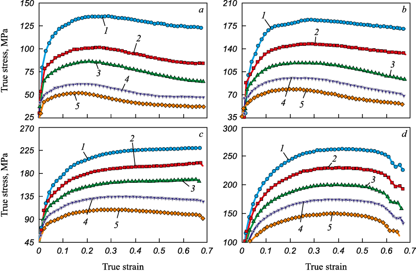
All researchers conducting multifactor analysis of hot deformation use the results of compression tests on cylindrical samples with a diameter of about 10 mm and a height-to-diameter ratio of ~1 to 2. In this study, the analysis was carried out using the results described in [12]. Yang-Hong Xiao and Cheng Guo, in their report, presented data from compression tests up to true strain values of ~1 at 1253 – 1453 K and compression rates of 0.01 – 10 s\(^–\)1 on samples of heat-resistant 12 % chromium steel 1Cr12Ni3Mo2VNbN. The shape of the initial deformation curves is shown in Fig. 1.
Fig. 1. Curves of hot compressive deformation in true coordinates |
By digitizing these curves using the Grafula program, an array of experimental data was obtained in the form of a table containing approximately 800 rows. In four columns, the table recorded data on deformation, stress, strain rate, and temperature for each experimental point (approximately 40 points for each of the 20 experimental curves). The independent variables were true strain φ′, and temperature Т (in K). The dependent variable was true stress S. A fragment of the initial data table is shown in Table.
Fragment of initial data array for analysis
|
Results and discussion
Taking into account the results of studiesdescribed above, the first step was to base the analysis on the generalized Arrhenius-type dependency (GM). Using the regress function from the Mathcad program, the values of the coefficients A, B, C, D were obtained in equation (1.1а). After reversing the logarithmic form of equation (1.1а) to the direct form (1.1b) the following equation was derived
| \[\begin{array}{c}\sigma = 5.633 \cdot {10^{ - 4}}{\varepsilon ^{0.077}}{{\dot \varepsilon }^{0.127}}\exp \left( { - \frac{{66.487}}{{RT}}} \right),\\(R = 8.315{\rm{J/mol}} \cdot {\rm{K}}).\end{array}\] | (1.1b) |
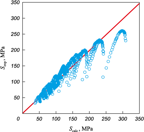
A visual assessment of the model’s quality was conducted by comparing the experimental values of S with the values calculated using the derived equation (1.1b) (Fig. 2).
Fig. 2. Comparison of calculated and experimental stress values |
To quantitatively assess the quality of the mathematical model, the sum of squared differences between the calculated and experimental stress values was computed, normalized to the mean stress value S using the formula
| \[Q = \frac{n}{{\sum S }}\sqrt {\sum {\frac{{{{\left( {{S_{{\rm{расч}}}} - {S_{{\rm{эксп}}}}} \right)}^2}}}{{n - 5}}} } .\] | (2) |
For the model in the form (1.1b), this value was approximately 14 %.
The comparison of the visual and quantitative assessments shows that, despite the small average deviation of the predicted values from the experimental ones, the model (1.1b) provides poor predictions for high-stress intervals (the final sections of the compression curves with large degrees of deformation) (Fig. 2).
In order to refine the assumed model, an analysis of individual deformation curves was conducted. Since the primary mathematical method for determining coefficients for the variables was linear regression analysis using the least squares method, the focus of the analysis was on linear equations with a logarithmic form of the variables. Preliminary trials (where “trial” refers to various mathematical formulations of the relationships between the variables) for determining equations that describe individual deformation curves (each of these curves was obtained at constant values of temperature and strain rate) showed that for most deformation curves, the equation of the form
| S = А(φ)\(^B\)10\(^C\)(φ) | (3) |
or, after logarithmization
| log(S) = A1 + B1 log(φ) + C1 (φ). | (3a) |
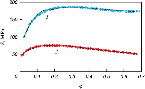
provides a good description. This representation allows obtaining Q values for individual curves in the range of 1.5 to 5 % (Fig. 3).
Fig. 3. Description of S – φ dependences with formula (3): |
The accuracy of the prediction improves even further when the expression (3a) is modified by including a multiplier in the form of the ratio of the strain degree φ to the logarithm of this value:
| \[\log (S) = A2 + B2\log (\varphi ) + C2(\varphi ) + \frac{{D2(\varphi )}}{{\log (\varphi )}}.\] | (4) |
The quality of such equations, evaluated by the parameter Q ranges from 0.5 to 1.7 % (Fig. 3), and the relationship between variables in its direct form (without logarithms) is described by the equation
| \[S = {\varphi ^{B3}}\exp \left[ {A3 + C3(\varphi ) + \frac{{D3(\varphi )}}{{\log (\varphi )}}} \right].\] | (4а) |
Further development of this model followed the next steps. In the deformation curves obtained from tests conducted at low temperatures and/or high strain rates, there is an extended section of significant stress increase after the yield point on the graphs, with a high strain hardening coefficient D = dS/dφ. Such a feature of the curve shape can be accounted for by introducing a third-degree polynomial of strain φ. Based on this logic, quadratic and cubic terms of the strain degree φ were added to the model in its logarithmic form:
| \[\begin{array}{c}\log (S) = A4 + B4\log (\varphi ) + C4\log {(\varphi )^2} + D4\log {(\varphi )^3} + \\ + E4(\varphi ) + \frac{{F4(\varphi )}}{{\log (\varphi )}}.\end{array}\] | (4в) |
In its direct form, this expression is described by the equation
| \[S = {\exp ^{A5 + E5(\varphi ) + \frac{{F5(\varphi )}}{{\log (\varphi )}}}}{\varphi ^{B5 + C5\log (\varphi ) + D5{{[\log (\varphi )]}^2}}}.\] | (4г) |
With this representation, the parameter Q for individual curves decreases from 0.3 to 1.0 %.
Taking all of the above into account, a modified mathematical model was developed to describe the complete dataset. The modifications to the model (1.1) in its logarithmic form (1.1a) were as follows:
– terms accounting for the degree of deformation φ and the strain rate φ′ were introduced (under the exponential sign) into the multiplier that accounts for the effect of deformation temperature;
– the mutual influence of independent factors on each other was accounted for by adding a multiplier (φφ′);
– dependencies on the square and cube of the strain degree φ were introduced through corresponding multipliers.
The general form of the equation for the relationship between variables, after being reduced to a linear form by logarithmization, looks as follows:
| \[\begin{array}{c}\log (S) = A + B\log (\varphi ) + C{[\log (\varphi )]^2} + D{[\log (\varphi )]^3} + \\ + E\log (\varphi ') + F\log (\varphi )\log (\varphi ') + G\left( {\frac{\varphi }{{\varphi '}}} \right) + \\ + \frac{{H + K\varphi + M\log (\varphi ) + N\log (\varphi ') + P\log (\varphi )\log (\varphi ')}}{T}.\end{array}\] | (5) |
Finding the coefficients A – P for equation (5), which ensures the minimum sum of squared differences between the calculated Scalc and experimental Sexp values, conducted using the Mathcad program, made it possible to obtain the desired equation for the relationship in the following form
| \[\begin{array}{c}\log (S) = - 0.738 - 1.311\log (\varphi ) - 0.564{[\log (\varphi )]^2} - \\ - 0.13{[\log (\varphi )]^3} + 0.584\log (\varphi ') - \\ - 8.779 \cdot {10^{ - 4}}\log (\varphi )\log (\varphi ') - 1.18 \cdot {10^{ - 3}}\left( {\frac{\varphi }{{\varphi '}}} \right) + \\ + \frac{{3.727 \cdot {{10}^3} + 82.351\varphi + 1.096 \cdot {{10}^{ - 3}}\log (\varphi )}}{T} + \\ + \frac{{593.8\log (\varphi ') + 76.6\log (\varphi )\log (\varphi ')}}{T},\end{array}\] | (6) |
which can be transformed into its direct form:
| \[\begin{array}{c}S = {10^{ - 0.738}}{(\varphi ')^{0.584}} \times \\ \times {\varphi ^{ - 1.311 - 0.564\log (\varphi ) - 0.131{{[\log (\varphi )]}^2} - 8.779 \cdot {{10}^{ - 4}}\log (\varphi ')}} \times \\ \times \exp \left[ {\frac{{8583.3 + 198.7\varphi + 2524\log (\varphi )}}{T} - } \right.\\ - \frac{{1367.5\log (\varphi ') + 176.4\log (\varphi )\log (\varphi ')}}{T} - \\ - \left. {2.718 \cdot {{10}^{ - 3}}\left( {\frac{\varphi }{{\varphi '}}} \right)} \right],\end{array}\] | (6а) |
or with the temperature component separated:
| \[\begin{array}{c}S = {10^{ - 0.738}}{(\varphi ')^{0.584}} \times \\ \times {\varphi ^{ - 1.311 - 0.564\log (\varphi ) - 0.131{{[\log (\varphi )]}^2} - 8.779 \cdot {{10}^{ - 4}}\log (\varphi ')}} \times \\ \times \exp \left[ { - 2.718 \cdot {{10}^{ - 3}}\left( {\frac{\varphi }{{\varphi '}}} \right)} \right] \times \\ \times \exp \left[ {\frac{{8583.3 + 198.7\varphi + 2524\log (\varphi )}}{T} - } \right.\\ - \left. {\frac{{1367.5\log (\varphi ') + 176.4\log (\varphi )\log (\varphi ')}}{T}} \right].\end{array}\] | (6б) |
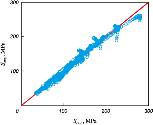
A graphical illustration of the agreement between the calculated and experimental values of S is shown in Fig. 4. The quality indicator of this model, Q = 6.1 %, is significantly better than that of the original model, both qualitatively and quantitatively (compare with Fig. 2).
Fig. 4. Comparison of calculated and experimental stress values |
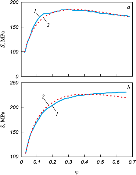
The obtained equation (6a) allows for predicting the shape of the deformation curve for various combinations of φ, φ′ and Т. Examples of such graphs, compared with experimental curves, are shown in Fig. 5. The presented graphs illustrate both “good” and “not-so-good” agreement between the calculated and experimental curves.
Fig. 5. Comparison of experimental (1) deformation curves |
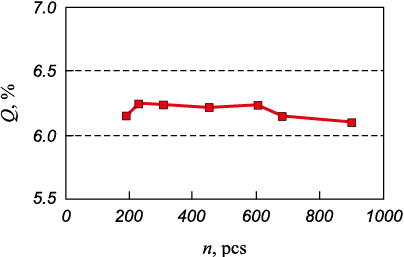
It is known from statistical theory [16] that increasing the sample size of experimental data can lead to improved accuracy in the description of a mathematical model (reducing its variance). To test this hypothesis, the number of original data points (the number of rows in the full matrix) was artificially reduced sequentially from ~900 to ~200, and the model quality indicator Q was recalculated. The results of these calculations are presented in Fig. 6. It can be seen that reducing the size of the experimental data sample by approximately 4 times (from 900 to 200) does not significantly affect the predictive quality of model (6а).
Fig. 6. Change in Q index of the generalized deformation model |
This unexpected result may reflect the fact that only a few characteristic points are decisive in shaping the modeled curve (in this respect, the methodology is similar to the aforementioned Johnson-Cook method).
An important test of the developed model’s functionality is its validation on other datasets. Using the methodology described above, the results of hot compression tests of materials from other groups were processed: heat-resistant nickel alloy Ni33Cr27Fe35Mo3.5Mn1Cu0.6 from the Inconel group [17], heat-resistant nickel alloys [18], and the Ni56Cr24Co14Mo0.5W1Nb1.5Al1.5Ti1.5 alloy from the Nimonic group [19], cobalt alloys [20; 21], ferritic heat-resistant Cr12 – Cr27 steels [22], heat-resistant 9 % chromium DUO steel [23], and steel 20Cr13 [24]. It was found that the developed type of mathematical model is applicable to these cases as well. It is implied that for all these cases, the nomenclature and form of the multipliers in the relationship formula are unified across all studied alloys, though the coefficients for these multipliers, naturally, differ. The predictive quality, evaluated by the Q, indicator ranged from 3 to 11 %.
Conclusions
A generalized mathematical model in multiplicative form has been proposed, which describes the relationship between stress, strain, strain rate, and temperature during large hot deformations (up to a true strain degree of 0.8), at temperatures ranging from 0.6 to 0.85Т/Тmelt) and strain rates between 0.01 and 10 s\(^–\)1. The model predicts deformation force with an accuracy of approximately 6 %, without relying on a priori (tabulated) or pre-determined structural, mechanical, or energy characteristics.
The multipliers used in the developed mathematical model reflect experimentally observed interdependencies between the independent variables (φ, φ′, Т) and the specific features of the deformation curves.
It has been established that this mathematical model is applicable to a wide range of metallic materials undergoing hot deformation, with predictive accuracy for deformation stress characteristics ranging from 3 to 11 %.
The obtained data allow for the analysis of not only test results with a fixed true strain rate φ′ – which is methodologically complex – but also results from experiments conducted using the traditional method with a constant nominal strain rate \(\dot \varepsilon \) where the true strain rate φ′ is not constant.
References
1. Shtremel’ M.A. Alloy Strength. Part 2. Deformation. Moscow: MISIS; 1997:527. (In Russ.).
2. Hollomon J.H. Tensile deformation. Trans AIME. 1945; 162:268–290.
3. Rosenberg V.M. Fundamentals of Heat Resistance of Metallic Materials. Moscow: Metallurgiya; 1973:328. (In Russ.).
4. Ludwigson D.C. Modified stress-strain relation for FCC metals and alloys. Metallurgical Transactions A. 1971;2(10): 2825–2828. https://doi.org/10.1007/BF02813258
5. Bershtein M.L., Zaimovskii V.A. Mechanical Properties of Metals. Moscow: Metallurgiya; 1979:496. (In Russ.).
6. Zener C., Hollomon J. H. Effect of strain rate upon plastic flow of steel. Journal of Applied Physics. 1944;15(1):22–32. https://doi.org/10.1063/1.1707363
7. Bird J.E., Mukherjee A.K., Dorn J.E. Experimental correlations between high-temperature creep behavior and structure. In: Quantitative Relation Between Properties and Microstructure. Brandon D.G., Rosen A. eds. Jerusalem University Press; 1969:255–342.
8. Johnson G.R., Cook W.H. Fracture characteristics of three metals subjected to various strains, strain rates, temperatures and pressures. Engineering Fracture Mechanics. 1985;21(1):31–48. https://doi.org/10.1016/0013-7944(85)90052-9
9. Sellars C.M., McTegart W.J. Cavity growth mechanisms during creep. Acta Metallurgical. 1966;14:1136–1138.
10. Sun C., Liu G., Zhang Q., Li R., Wang L. Determination of hot deformation behavior and processing maps of IN 028 alloy using isothermal hot compression test. Materials Science and Engineering: A. 2014;595:92–98. https://doi.org/10.1016/j.msea.2013.10.051
11. Fang B., Ji Z., Liu M., Tian G., Jia C., Zeng T., Benfu HU, Wang C. Study on constitutive relationships and processing maps for FGH96 alloy during two-pass hot deformation. Materials Science and Engineering: A. 2014;590:255–261. https://doi.org/10.1016/j.msea.2013.10.034
12. Xiao Y.-H., Guo C. Constitutive modeling for high temperature behavior of 1Cr12Ni3Mo2VNbN martensitic steel. Materials Science and Engineering: A. 2011;528(15): 5081–5087. https://doi.org/10.1016/j.msea.2011.03.050
13. Zerilli F.J., Armstrong R.W. Dislocation-mechanics-based relations for material dynamics calculations. Journal of Applied Physics. 1987;61(5):1816–1825. https://doi.org/10.1063/1.338024
14. Belomyttsev M.Yu. Experimental analysis of creep regularities of high-temperature ferritic-martensitic steel. Deformatsiya i razrushenie materialov. 2019;(10):31–41. (In Russ.).
15. Belomyttsev M.Yu., Molyarov V.G. Creep resistance of ferritic-martensitic steel 16Cr12MoWSiVNbB (EP-823). Izvestiya. Ferrous Metallurgy. 2019;62(4):290–302. (In Russ.). https://doi.org/10.17073/0368-0797-2019-4-290-302
16. Melnichenko A.S. Statistical Analysis in Metallurgy and Materials Science: Textbook. Moscow: MISIS; 2009:268. (In Russ.).
17. Wang L., Liu F., Cheng J.J., Zuo Q., Chen C.F. Hot deformation characteristics and processing map analysis for Nickel-based corrosion resistant alloy. Journal of Alloys and Compounds. 2015;623:69–78. https://doi.org/10.1016/j.jallcom.2014.10.034
18. Pan Q.L., Li B., Wang Y., .Zhang Y.W., Yin Z.M. Characterization of hot deformation behavior of Ni-base superalloy Rene’41 using processing map. Materials Science and Engineering: A. 2013;585:371–378. https://doi.org/10.1016/j.msea.2013.07.066
19. Wu Y., Zhang M., Xie X., Dona J., Lin F., Zhao S. Hot deformation characteristics and processing map analysis of a new designed nickel-based alloy for 700 °C A-USC power plant. Journal of Alloys and Compounds. 2016;656:119–131. https://doi.org/10.1016/j.jallcom.2015.09.219
20. Kumar V.A., Gupta R.K., Murty S.V.S. Narayana, Prasad A.D. Hot workability and microstructure control in Co20Cr15W10Ni cobalt based superalloy. Journal of Alloys and Compounds. 2016;676:527–541. https://doi.org/10.1016/j.jallcom.2016.03.186
21. Kartica Ika, Matsumoto H., Chiba A. Deformation and microstructure evolution in Co-Ni-Cr-Mo superalloy during hot working. Metallurgical and Materials Transactions A. 2009;40:1457–1468. https://doi.org/10.1007/s11661-009-9829-x
22. Mehtonen S.V., Karjalainen L.P., Porter D.A. Modeling of the high temperature flow behavior of stabilized 12 – 27wt% Cr ferritic stainless steels. Materials Science and Engineering: A. 2014;607:44–52. https://doi.org/10.1016/j.msea.2014.03.124
23. Zhang G., Zhou Z., Sun H., Zou L., Wang M., Li S. Hot deformation behavior and processing map of a 9Cr ferritic/martensitic ODS steel. Journal of Nuclear Materials. 2014;455(1-3):139–144. https://doi.org/10.1016/j.jnucmat.2014.05.043
24. Akhmed’anov A.M., Rushchits S.V., Smirnov M.A. Physical and numerical modeling of hot deformation behaviour of 20Kh13 steel. Bulletin of SUSU. Series “Metallurgy”. 2013;13(2):116–124. (In Russ.).
About the Author
M. Yu. BelomyttsevRussian Federation
Mikhail Yu. Belomyttsev, Dr. Sci. (Eng.), Prof. of the Chair “Metallography and Physics of Strength”
4 Leninskii Ave., Moscow 119049, Russian Federation
Review
For citations:
Belomyttsev M.Yu. Type of generalized mathematical model for describing large hot deformations. Izvestiya. Ferrous Metallurgy. 2024;67(5):616-624. https://doi.org/10.17073/0368-0797-2024-5-616-624


