Scroll to:
Using machine learning tools to study flow stress of tube steels under laboratory conditions and according to industrial rolling data
https://doi.org/10.17073/0368-0797-2023-1-70-79
Abstract
Studying the flow stress of various steel grades is one of the key issues for the viable operation of automation systems which support the production of rolled products with the required precision based on geometrical properties. A knowledge of flow stress is also important for the design of rolling mill equipment. The properties of flow stress are published mainly in the form of coefficients of various equations (for instance, the Hansel–Spittel equation). However, these equations are quite often limited in terms of process variables where they provide accessible result. It also should be taken into account that the existing rolling industry fabricates tens of steel grades, the chemical composition of which can vary in wide range depending on final thickness of the rolled products, customer requirements, or on the basis of economic considerations. Studies of the rheological properties of such amount of materials under laboratory conditions is expensive, time and labor consuming and published data does not provide data completeness. This work demonstrates that, using data from industrial rolling mills and methods of machine learning, it is possible to obtain data on material rheology with satisfactory precision. This allows laboratory studies to be avoided. Similar studies are possible due to high intensity of various sensors and instrumentation in modern rolling mills. The results of industrial data were compared with flow stress measured by Gleeble. On the basis of this comparison the model was trained using gradient boosting in order to consider peculiarities of industrial production process.
Keywords
For citations:
Zinyagin A.G., Muntin A.V., Kryuchkova M.O. Using machine learning tools to study flow stress of tube steels under laboratory conditions and according to industrial rolling data. Izvestiya. Ferrous Metallurgy. 2023;66(1):70-79. https://doi.org/10.17073/0368-0797-2023-1-70-79
Introduction
The design calculations of rolling equipment and development of new process modes are based on process power parameters (PPP), mainly rolling force. In general terms, the calculation equations of contact stresses include directly the flow stress. Therefore, the precision of its detection influences directly on the PPP calculation error. Despite the available theoretical and empirical equations, which describe the influence of temperature, the strain rate and velocity on flow stress, their precision is not always acceptable during calculations for steel of new chemical composition. Therefore, the precise value of flow stress of steels and alloys of certain chemical composition should be reasonably determined by experimental means.
Several determination methods of flow stress are available, such as tension, compression, cylinder torsion, and others. Flow stress determined under compression, tension, and torsion can be used with certain assumptions in calculations of contact pressure during rolling. This is attributed to differences under deformation development, under temperature conditions, and other factors [1].
Direct determination of flow stress can be established while rolling. The method of basis pressures can be used with this aim [2]. However, such an approach is more labor intensive and requires sufficiently powerful rolling equipment. In addition, the rolling of one sample at once and the same deformation provides sufficiently less data than compression tests, which present data in the range of true strain from 0 to ~1.
A significant expansion of knowledge about flow stress of metal under actual industrial conditions can be achieved by using statistic methods of processing large data arrays obtained from sensors and control systems of rolling mills. One year of operation of sheet rolling mill provides information of about two million passes [3, 4].
Using the above-mentioned values and validating the results by compression tests (Gleeble), it is possible to develop calculation procedure of flow stress on the basis of industrial data without supplementary laboratory studies.
Modern rolling mills are intensively equipped with sensors which allow very precise detection of actual process parameters. The data obtained is collected at a high sampling rate, accumulated in files, and can be used for advanced statistical analysis. It should be mentioned that due to high scatter of parameters influencing the process, the data analysis from industrial rolling mills using classical methods is very difficult. In such cases machine learning methods are widely applied for data cleaning and highlighting of key features of the running processes. In other countries, neural networks are used for forecasting the physical properties of hot rolled thick sheet (flow stress), rolling force, and other parameters. Using such models, it is possible to significantly decrease expenses of studies during development of new products.
For example, in [5] the neural network is used as adaptation of the various calculation methods of rolling force (Sims, Tselikov) in a single rolling mill. The initial data are both the standard rolling conditions (temperature, compression, rolling geometry, and so on), and the calculated forces using the aforementioned procedures.
The researchers in [6 – 8] use machine learning methods for description of curves obtained using Gleeble. This approach allows more precise data to be obtained than by classical approaches.
In [9], the use of general rolling parameters and a fully connected neural network, the authors successfully forecast rolling force and moment.
In [10 – 14] the simulation of the plastic properties of various alloys at high temperatures are considered by means of fully connected neural networks. The features of this approach are discussed here.
Machine learning is also used for forecasting phase transformations during rolling and analysis of material properties, for which analytical dependences were not developed [15 – 19].
The aim of this work is to determine the thermo-mechanical coefficients for calculating flow stress of selected steel on the basis of laboratory and industrial studies. In order to achieve the formulated target, various steel grades were analyzed by means of compression and rolling tests, their rheological properties were determined, and the model was proposed in accordance with machine learning methods for calculating coefficients of the Hansel–Spittel equation.
Analyzed materials, procedures and equipment
Four variants of chemical composition of steels were considered in this work used for production of rolled products for pipes, grade K52 – K60. The chemical composition of the steels considered is summarized in Table 1. Steels 1 – 4 are mentioned without grade specification in order to preserve confidentiality.
Table 1. Chemical composition of the considered samples, (wt. %)
| ||||||||||||||||||||||||||||||||||||||||||||||||||||||||||||
For steel 1, the tests on the Gleeble facility were carried out for basic chemical composition. However, the data from industrial rolling mill was analyzed using several variants of chemical composition, the main difference being the content of niobium.
Compression test is one of the most popular methods used to determine rheological properties. This method allows carry out tests with high strain (about 60 %) and strain rate up to 20–30 s–1 to be carried out. In this work the compression tests were carried out on the Gleeble facility. A typical sample was a cylinder with the diameter of 10 mm and the height of 15 mm.
One drawback of the method is changes in the sample shape upon deformation from cylindrical to barrel type. To reduce barrel distortion, a lining made of graphite and tantalum foils was used between the dies and the sample (Fig. 1).
Fig. 1. External view of the Gleeble 3800 test block (a), strain layout (b) and sample for the experiment (c) |
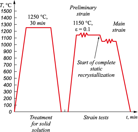
The samples were tested in the temperature range of 750 – 1150 °C (with the increment of 50 °C) at three strain rates: 0.1; 1, and 10 s–1. Therefore, 30 tests were carried out for each steel grade. To obtain reliable results, a thermal cycle was applied consisting of:
– treatment for solid solution, in order to dissolve carbonitride particles;
– heating to 1150 °С;
– preliminary strain (ε = 0.1);
– holding up to complete static recrystallization;
– cooling to test temperature;
– main strain and quenching (Fig. 2).
Fig. 2. Test thermal cycle |
As a consequence of tests a set of discrete curves was obtained: true strain – true stress σ(ε).
Samples for tests on the Gleeble facility were fabricated from industrial rolled products of the respective steel grades.
Results and discussion
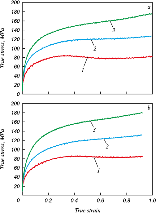
Partial test results of uniaxial compression of samples with the diameter of 10 mm and the height of 15 mm for steels 2 and 4 at the strain rate of 1 s–1 are shown in Fig. 3.
Fig. 3. Effect of temperature 1150 (1), 1050 (2), 950 °С (3) |
The curves obtained can be subdivided into two types. The first type describe strain comprised simultaneously of strengthening and softening, and their ratio determine the form of the curve. At the same time, softening starts with very little strain dynamic. This tries to restore a previous state due to redistribution of dislocations. After achieving equilibrium, the stress remains actually the same with increase in strain degree. The curves of the first type can be observed in a significant part of the considered range of temperature and strain parameters. For example, for steel 4 in Fig. 3 – these are the curves at 1050 and 950 °C.
The curves of the second type are obtained due to low activation energy under the given strain conditions. Dynamic recrystallization starts after achieving critical density of dislocations at certain strain. If the dynamic recrystallization starts before the achievement of equilibrium state between strengthening and softening, then the following is observed decrease in stress with strain increase. The curves of the second type are observed in the region of higher temperatures and low strain rates. In Fig. 3, these are the curves at 1150 °C.
As mentioned above, the results of compression tests on the Gleeble facility are true stress as a function of true strain. However, this dependence cannot be directly applied to the calculation of flow stress in strain source upon rolling due to discreteness of the curves. For correct use it is required to convert true stress into average stress using the following equation [20]
| \({\sigma _{\rm{c}}} = \frac{{\int_{{\varepsilon _1}}^{{\varepsilon _2}} {\sigma (\varepsilon )d\varepsilon } }}{{{\varepsilon _2} - {\varepsilon _1}}}\), | (1) |
where σ(ε) is the stress curve obtained on Gleeble facility; ε1 , ε2 are the initial and final value of true strain at the segment.
Also, for ease of calculation of rolling modes, the true strain can be converted into a relative one using the following equation
| εrel = 1 – e–ε. | (2) |
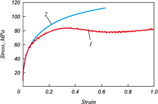
Figure 4 illustrates the curves before and after conversion.
Fig. 4. Comparison of true (1) and average (2) stresses |
The influence of strain degree, strain rate and temperature obtained in the form of curves are often described by the Hansel–Spittel equation [1]
| \(\sigma = {A_1}{A_2}{A_3}{\varepsilon ^{{m_1}}}{u^{{m_2}}}{e^{ - {m_3}T}}{\sigma _{\rm{b}}}\), | (3) |
where A1 , A2 , A3 , m1 , m2 , m3 are the empirical coefficients; e is the relative strain; u is the strain rate; T is the metal temperature; σb is the average flow stress at basic test parameters (in this work taken equal to ε = 10 %, u = 1 s–1, Т = 900 °С).
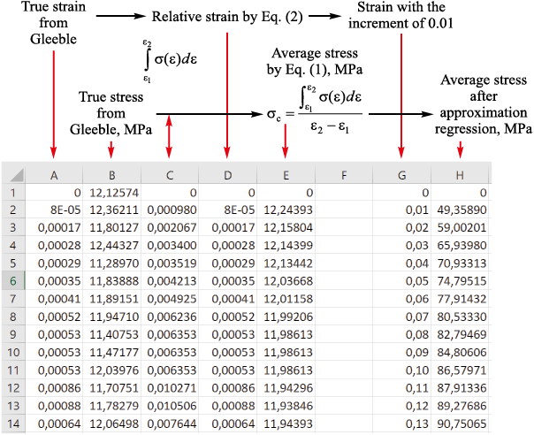
To eliminate the influence of variations, all the curves were reduced to one basis in terms of strains. The conversion procedure is illustrated in Fig. 5. On the basis of the obtained data linear regression analysis was carried out for Eq. (3), and the result of the approximation was the coefficients m0 = ln (A1 A2 A3σb ), m1 , m2 , m3
Fig. 5. Conversion algorithm of true stress – true strain to average flow stress – strain |
| \(\ln \,\sigma = \ln \,\left( {{A_1}{A_2}{A_3}\,{\varepsilon ^{{m_1}}}{u^{{m_2}}}{e^{-{m_3}T}}{\sigma _{\rm{b}}}\,} \right)\); | (4) |
| \(\ln \,\sigma = \ln \,\left( {{A_1}{A_2}{A_3}{\sigma _{\rm{b}}}} \right) + {m_1}\ln \,\varepsilon + {m_2}\ln u - {m_3}T\). | (5) |
As a result, the following equations were obtained for the considered steel grades:
| σsteel 1 = 2245ε 0.2864 u 0.1001 e –0.00274T ; | (6) |
| σsteel 2 = 2827ε 0.3334 u 0.1097 e –0.00288T ; | (7) |
| σsteel 3 = 1818ε 0.2544 u 0.1119 e –0.00262T ; | (8) |
| σsteel 4 = 2649ε 0.3142 u 0.0989 e –0.00285T . | (9) |
Another possible method of obtaining data on flow stress is to analyze results from industrial rolling mills. In comparison with laboratory conditions, the industrial environment can entail higher strain degrees, complicated strain – stress states, significant temperature heterogeneity with large size of workpiece, non-standard friction conditions and other factors, making obtaining of precise results more difficult.
In this paper it is proposed to use reverse calculations of flow stress from rolling force using classical approaches [2], based on data from industrial rolling mill 5000. Then, to calculate the coefficients of the equation of the Hansel–Spittel equation. The calculations were based on each separate pass (the data from more than 310 thousand passes were studied).
This work analyzed only roughing stage. The rolling width was from 2500 to 4500 mm, and the thickness was from 50 to 350 mm. The remaining parameters in the learning sampling were varied as follows: strain from 0.02 to 0.27; strain rate from 0.42 to 5.93 s–1, temperature from 920 to 1150 °C.
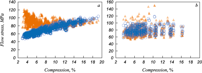
The flow stress was calculated using the data from rolling mill (thickness, compression, diameter of rolls, temperature and other process variables). This was based on a procedure similar but inverse to calculations of rolling force according to Tselikov [2]. Based on the example of steel 1, let us consider the form of the dependence obtained in comparison with data from the Gleeble facility (Fig. 6).
Fig. 6. Comparison of calculated flow stress using industrial data ( |
At compressions more than 10 %, the properties determined by the two methods are identical, herewith, up to 10 % the flow stress from the rolling mill significantly exceed the data from Gleeble facility. We believe that this can be attributed to the features of recrystallization of the austenitic grain, as well as to errors in back calculation of flow stress when classical theories of rolling are used. It should be mentioned that this effect is observed not for all variants of steel grades but mainly for those containing niobium.
To consider this, a model was developed on the basis of gradient boosting (Catboost library). As a learning sampling, the data for steel 1 was taken for different chemical compositions (7 variants in total). 15 features were used: chemical composition, compression; time before passes; strain rate; rolling thickness; temperature and number of passes. The relative difference between the calculated flow stress from the rolling mill and the data from the Gleeble facility was taken as the targeted feature. The values obtained were subdivided into testing and learning samplings in the ratio of 75 – 25 %.
The RMSE (root mean square error) was taken as the loss function. In addition, the R2 metrics, coefficient of determination, was used for quality estimation of the obtained forecasted data.
The model was traoned by selection of optimum parameters using grid_search, and carried out as follows:
– ‘learning_rate’: [0.05, 0.1, 0.3];
– ‘depth’ (tree depth, that is, number of partitions before forecast): [4, 6, 8, 10];
– ‘l2_leaf_reg’ (coefficient of regularization l2): [4, 6, 8].
The best parameters were as follows: ‘depth’ = 8, ‘learning rate’ = 0.3, ‘l2_leaf_reg’ = 6. The obtained precision of the model by the RMSE metrics is 3.2 MPa, R2 0.97.
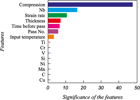
The most important features are illustrated in Fig. 7. As can be seen, the most important are the features directly influencing of strengthening and softening, namely: strain, niobium content, strain rate.
Fig. 7. Significance level of the model features |
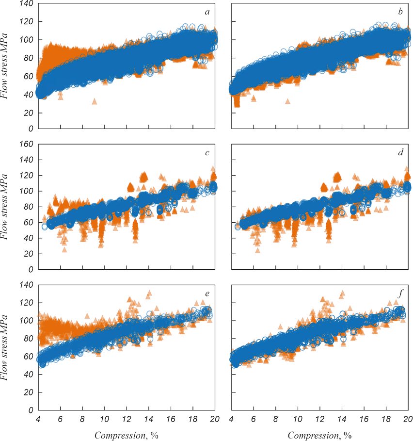
The model performance was then tested for steels 2 – 4. Dependences of flow stress based on data from rolling mill before and after application of the model to the mentioned steels are shown below.
As can be seen in Fig. 8 and Table 2, application of the model significantly improves the accuracy of determining flow stress. For steel 2, the RMSE parameter decreased by 6.5 times, and the R2 parameter from negative value increased to 0.94. For steels 3 and 4, the result was less precise – RMSE: 5.37 and 5.88 MPa, R2: 0.89 and 0.85.
Fig. 8. Flow stress as a function of compression for steel 2 (а, b), 3 (c, d), 4 (e, f ) |
Table 2.Comparison of the determination precision of flow stress
|
On the basis of the data obtained, the coefficients of the Hansel–Spittel equation were calculated. Comparison with the data from the Gleeble is shown in Table 3. The coefficients differ mainly due to the features of description method of stress – strain curves. Therefore, it would be reasonable to compare not single coefficients but their combined action, that is, calculated flow stress. As can be seen in Table 2, the absolute calculated values by two procedures differ by 3 – 7 %.
Table 3. Comparison of the HenselSpittel coefficients according to the data
|
Therefore, application of the obtained coefficients provides satisfactory precision of determination of flow stress in the above-mentioned range of process variables. The models of flow stress obtained by statistical processing of industrial data can be applied for engineering calculations of PPP.
Conclusions
The flow stress of four steel grades with various chemical compositions measured by Gleeble was compared with the measurements at rolling mill 5000.
The discrete curves obtained in the experiments were approximated, and the coefficients of the Hansel–Spittel equation were determined.
Показано, что при расчете сопротивления деформации на основе промышленных данных, при обжатиях менее 10 % наблюдается расхождение с данными, полученными на установке Gleeble.
It was demonstrated that upon calculation of flow stress on the basis of industrial data at compression less than 10%, the data does not agree with those obtained at the Gleeble facility.
In order to account this phenomenon, it was proposed to use the machine learning model based on gradient boosting (Catboost library) . The best model parameters were as follows: ‘depth’ = 8, ‘learning_rate’ = 0.3, ‘l2_leaf_reg’ = 6. The model learning was based on industrial and laboratory data of one and the same steel grade with several variants of chemical composition. The obtained precision of the model with test selection by the RMSE metrics equals to 3.2 MPa, R2 is 0.97.
The use of this model allowed to achieve the precision of flow stress determination to be increased significantly. For steel 2, the RMSE parameter decreased by 6.5 times. The R2 parameter from negative, increased to 0.94. For steels 3 and 4, the results were less precise – RMSE: 5.37 and 5.88 MPa, R2: 0.89 and 0.85.
A comparison of the industrial values of flow stress with the data obtained by Gleeble demonstrated close results and the capability to use the described approach to analyze steel flow stress based on industrial data.
References
1. Hensel A., Spittel T. Kraft- und Arbeitsbedarf bildsamer Formgebungsverfahren. Leirzig: Verlag; 1978. (In Germ.).
2. Nikitin G.S. Theory of Longitudinal Continuous Rolling. Moscow: Bauman MSTU; 2009: 203. (In Russ.).
3. Muntin A.V., Kurenkov Yu.M., Kolesnikov A.G. С Modern technological solutions and equipment for the production of ultra-thin hot-rolled strip. Proizvodstvo prokata. 2016; (8): 13–21. (In Russ.).
4. Muntin A.V. Advanced technology of combined thin slab continuous casting and steel strip hot rolling. Metallurgist. 2019; 62 (9–10): 900–910. https://doi.org/10.1007/s11015-019-00747-5
5. Vannucci M., Colla V., Dimatteo A. Improving the estimation of mean flow stress within hot rolling of steel by means of different artificial intelligence techniques. IFAC Proceedings Volumes. 2013; 46(9): 945–950. https://doi.org/10.3182/20130619-3-RU-3018.00326
6. Thakur S.K., Das A.K., Jha B.K. Development of an integrated flow stress and roll force models for plate rolling of microalloyed steel. Steel Research International. 2022; 93(2): 2100479. https://doi.org/10.1002/srin.202100479
7. Murugesan M., Yu J., Jung K., Cho S., Bhandari K.S., Chung W., Lee C. Supervised machine learning approach for modeling hot deformation behavior of medium carbon steel. Steel Research International. 2023; 93(1): 2200188. https://doi.org/10.1002/srin.202200188
8. Aghasafari P., Abdi H., Salimi M. Artificial neural network modeling of flow stress in hot rolling. ISIJ International. 2014; 54(4): 872–879. https://doi.org/10.2355/isijinternational.54.872
9. Bagheripoor M., Bisadi H. Application of artificial neural networks for the prediction of roll force and roll torque in hot strip rolling process. Applied Mathematical Modelling. 2013; 37(7): 4593–4607. https://doi.org/10.1016/j.apm.2012.09.070
10. Murugesan M., Sajjad M., Jung D.W. Hybrid machine learning optimization approach to predict hot deformation behavior of medium carbon steel material. Metals. 2019; 9(12): 1315. https://doi.org/10.3390/met9121315
11. Moon I.Y., Jeong H.W., Lee H.W., Kim S.-J., Oh Y.-S., Jung J., Oh S., Kang S.-H. Predicting high temperature flow stress of nickel alloy A230 based on an artificial neural network. Metals. 2022; 12(2): 223. https://doi.org/10.3390/met12020223
12. Cao G.-M., Gao Z.-W., Gao X.-Y. Predicting flow stress of Ni steel based on machine learning algorithm. Proceedings of the Institution of Mechanical Engineers, Part C: Journal of Mechanical Engineering Science. 2022; 236(8): 4253–4266. https://doi.org/10.1177/09544062211048175
13. Lin Y.C., Zhang J., Zhong J. Application of neural networks to predict the elevated temperature flow behavior of a low alloy steel. Computational Materials Science. 2008; 43(4): 752–758. https://doi.org/10.1016/j.commatsci.2008.01.039
14. Stendal J.A., Bambach M., Eisentraut M., Sizova I., Weiß S. Applying machine learning to the phenomenological flow stress modeling of TNM-B1. Metals. 2019; 9(9): 220. https://doi.org/10.3390/met9020220
15. Versino D., Tonda A., Bronkhorst C.A. Data driven modeling of plastic deformation. Computer Methods in Applied Mechanics and Engineering. 2017; 318: 981–1004. https://doi.org/10.1016/j.cma.2017.02.016
16. Wang L.-y., Li L., Zhang Zh.-h. Accurate descriptions of hot flow behaviors across β transus of Ti-6Al-4V alloy by intelligence algorithm GA-SVR. Journal of Materials Engineering and Performance. 2016; 25: 3912–3923. https://doi.org/10.1007/s11665-016-2230-1
17. Zhang X., Zhi C., Wang Y., Li Y. Constitutive parameters identification of Q345E steel during hot deformation with inverse methods based on teaching–learning-based optimisation algorithm. Materials Research Innovations. 2015; 19(8): 634–638. https://doi.org/10.1179/1432891715Z.0000000001874
18. Santosh S., Sampath V., Mouliswar R.R. Hot deformation characteristics of NiTiV shape memory alloy and modeling using constitutive equations and artificial neural networks. Journal of Alloys and Compounds. 2022; 901: 163451. https://doi.org/10.1016/j.jallcom.2021.163451
19. Bambach M., Gerster S., Herty M. Online data assimilation of a hybrid flow stress model by particle filtering. CIRP Annals. 2021; 70(1): 255–260. https://doi.org/10.1016/j.cirp.2021.04.002
20. Zinyagin A.G. Improving the processes of rolling and cooling of sheets from pipe steel on mill-5000: Cand. Tech. Sci. Diss. Moscow; 2014: 159. (In Russ.).
About the Authors
A. G. ZinyaginRussian Federation
Aleksei G. Zinyagin, Cand. Sci. (Eng.), Assist. Prof., Bauman Moscow State Technical University (Bauman MSTU), Chief Innovation Specialist, JSC “Vyksa Metallurgical Plant”
5/1 Baumanskaya 2-ya Str., Moscow 105005, Russian Federation
45 Br. Batashevykh Str., Vyksa, Nizhny Novgorod Region 607060, Russian Federation
A. V. Muntin
Russian Federation
Aleksandr V. Muntin, Cand. Sci. (Eng.), Assist. Prof. of the Chair “Rolling Equipment and Technologies”, Bauman Moscow State Technical University (Bauman MSTU); Deputy Director for Research Activities, JSC “Vyksa Metallurgical Plant”
5/1 Baumanskaya 2-ya Str., Moscow 105005, Russian Federation
45 Br. Batashevykh Str., Vyksa, Nizhny Novgorod Region 607060, Russian Federation
M. O. Kryuchkova
Russian Federation
Mariya O. Kryuchkova, Senior Lecturer
5/1 Baumanskaya 2-ya Str., Moscow 105005, Russian Federation
Review
For citations:
Zinyagin A.G., Muntin A.V., Kryuchkova M.O. Using machine learning tools to study flow stress of tube steels under laboratory conditions and according to industrial rolling data. Izvestiya. Ferrous Metallurgy. 2023;66(1):70-79. https://doi.org/10.17073/0368-0797-2023-1-70-79


